library(tidyverse)

MergedDataDF<-read.csv("https://strath-my.sharepoint.com/:x:/g/personal/xanne_janssen_strath_ac_uk/EYaktlzmqLZOomPrXuaZrp8By9S5DNy_JepWQNZT-cy9ZA?download=1")
PopulationDF<-read.csv("https://strath-my.sharepoint.com/:x:/g/personal/xanne_janssen_strath_ac_uk/EW7K4EUEA59FpIBJmZk8GzoB2Hv_hp-FWZw3XzQXywWgaQ?download=1")13 Practical 5b: Exploratory data analysis in R
During this practical you will recap conducting exploratory analysis in R. We will use the cleaned data files we used during practical 3.
13.1 Exercises
The files for the exercises can be found here.
Exercise 1: Open P3_output1.csv and name the dataframe MergedDataDF. Open P3_ouput2.csv and name the dataframe Population.
Show the answer
13.2 Exploratory data analysis
Let’s first check the average height, weight and age of our sample.
Exercise 2: Can you create a df named DatabyAthletePerYear which displays the Sex, Age, Height, Weight, Number of Events taken part in, Number of Medals, and Sport of the athlete by year of participation? Also rename Name to Athlete
Show the answer
#Note how i use reframe here, this is the new version of summarise - you will still see me use summarise occasionally
DatabyAthletePerYearDF <- MergedDataDF %>%
  group_by(Name, Year) %>%
    reframe(Sex=max(Sex),
              Age = mean(Age, na.rm = TRUE),
              Height = mean(Height, na.rm=TRUE),
              Weight = mean(Weight, na.rm=TRUE),
              NumberEvents = sum(!is.na(Event)),
              NumberMedals = sum(Medal=="Gold"|Medal=="Silver"|Medal=="Bronze"),
              Sport=toString(unique(Sport)),
              Country=max(Country))%>%
#Renaming this column in preperation for the next steps
  rename(Athlete=Name)
Exercise 3: From here can you now create an df named DatabyAthleteAvg which shows an overview of the athlete over the years (i.e. one row per athlete)?
Show the answer
DatabyAthleteAvgDF <- DatabyAthletePerYearDF %>%
   group_by(Athlete)%>%
  reframe(Year=toString(unique(Year)),
         NumberOlympics = sum(!is.na(Year)),
         Age = mean(Age, na.rm=TRUE),
         Height = mean(Height, na.rm=TRUE),
         Weight = mean(Weight, na.rm=TRUE),
         NumberMedals=sum(NumberMedals),
         Sport=toString(unique(Sport)),
         Country=max(Country))
Now lets visualize some of this data using overview tables. We will use the “flextable” package to create our summary table (install and load if not already done so). We will show age, height, weight, total number of events, number of medals, number of athletes, gender split, total number of sports and countries in a table for 1988 and 2016.
Show the code
library(flextable)
# First we will calculate the outcomes we want in a df called table
SummaryStatsDF<-DatabyAthletePerYearDF %>%
#filter for relevant years
  filter(Year==1988 | Year == 2016) %>%
# group day by year
  group_by(Year) %>%
# calculate outcomes
  reframe(Age_avg= mean(Age, na.rm=TRUE),
          Age_sd=sd(Age, na.rm=TRUE),
          Height_avg= mean(Height, na.rm=TRUE),
          Height_sd=sd(Height, na.rm=TRUE),
          Weight_avg= mean(Weight, na.rm=TRUE),
          Weight_sd=sd(Weight, na.rm=TRUE),
          NumberEvents_avg= mean(NumberEvents, na.rm=TRUE),
          NumberEvents_sd=sd(NumberEvents, na.rm=TRUE),
          NumberMedals_sum=sum(NumberMedals,na.rm=TRUE),
          Athlete_freq=n_distinct(Athlete, na.rm=TRUE),
          Sport_freq=n_distinct(Sport, na.rm=TRUE),
          Country_freq=n_distinct(Country, na.rm=TRUE))

# Create individual year tables we will use in a second
Summary1988 <- SummaryStatsDF %>% filter(Year == 1988)
Summary2016 <- SummaryStatsDF %>% filter(Year == 2016)

# Design the table
TableDF <- tibble(
  Variable = c("Age","Height", "Weight", "Number of Events", "Number of Medals", "Number of Athletes", "Sports", "Countries"),
# totals should only include those were totals are relevant (i.e. medals, athletes, sports, countries)
  Total88 = c(NA, NA, NA, NA, Summary1988$NumberMedals_sum, Summary1988$Athlete_freq, Summary1988$Sport_freq,Summary1988$Country_freq),
# averages include those were averages and sds are relevant (i.e. height, weight, number of events athletes participated in)
  Average88 = c(Summary1988$Age_avg, Summary1988$Height_avg,Summary1988$Weight_avg, Summary1988$NumberEvents_avg, NA, NA, NA, NA),
  SD88 = c(Summary1988$Age_sd, Summary1988$Height_sd,Summary1988$Weight_sd, Summary1988$NumberEvents_sd, NA, NA, NA, NA),
# do the same for 2016
  Total16 = c(NA, NA, NA, NA, Summary2016$NumberMedals_sum, Summary2016$Athlete_freq, Summary2016$Sport_freq,Summary2016$Country_freq),
  Average16 = c(Summary2016$Age_avg, Summary2016$Height_avg,Summary2016$Weight_avg, Summary2016$NumberEvents_avg, NA, NA, NA, NA),
  SD16 = c(Summary2016$Age_sd, Summary2016$Height_sd,Summary2016$Weight_sd, Summary2016$NumberEvents_sd, NA, NA, NA, NA)
)

# plot table as a flextable.
TableFig <- flextable(TableDF) %>%
  colformat_double() %>%
  separate_header() %>%
  theme_vanilla() %>%
  align(align = "center", part = "all") %>%
  valign(valign = "center", part = "header") %>%
  autofit()

TableFig
Variable | Total88 | Average88 | SD88 | Total16 | Average16 | SD16 |
|---|---|---|---|---|---|---|
Age | 24.7 | 5.0 | 26.4 | 5.4 | ||
Height | 177.1 | 10.5 | 176.7 | 11.2 | ||
Weight | 72.6 | 14.7 | 71.9 | 16.1 | ||
Number of Events | 1.5 | 1.0 | 1.2 | 0.7 | ||
Number of Medals | 1,845 | 2,023 | ||||
Number of Athletes | 9,860 | 11,174 | ||||
Sports | 58 | 39 | ||||
Countries | 157 | 206 |
TableFig <- add_header_row(TableFig, values = c("", "1988", "2016"), colwidths = c(1,3, 3))%>%
  set_header_labels(
    Variable = "",
    Total88 = "Total",
    Average88 = "Average",
    SD88 = "SD",
    Total16 = "Total",
    Average16 = "Average",
    SD16 = "SD") %>%
  bold(j=1,bold=TRUE,part="body")

TableFig
1988 | 2016 | |||||
|---|---|---|---|---|---|---|
Total | Average | SD | Total | Average | SD | |
Age | 24.7 | 5.0 | 26.4 | 5.4 | ||
Height | 177.1 | 10.5 | 176.7 | 11.2 | ||
Weight | 72.6 | 14.7 | 71.9 | 16.1 | ||
Number of Events | 1.5 | 1.0 | 1.2 | 0.7 | ||
Number of Medals | 1,845 | 2,023 | ||||
Number of Athletes | 9,860 | 11,174 | ||||
Sports | 58 | 39 | ||||
Countries | 157 | 206 | ||||
#If we wanted to add significance or a footnote that's also possible by adding text below (this add significance * for age.
TableFig <-footnote(TableFig, i=1, j=c(3,6),
           value=as_paragraph(c("Significant at p<0.05")),
           ref_symbols=c("*"),
           part="body",inline=TRUE)
TableFig
1988 | 2016 | |||||
|---|---|---|---|---|---|---|
Total | Average | SD | Total | Average | SD | |
Age | 24.7* | 5.0 | 26.4* | 5.4 | ||
Height | 177.1 | 10.5 | 176.7 | 11.2 | ||
Weight | 72.6 | 14.7 | 71.9 | 16.1 | ||
Number of Events | 1.5 | 1.0 | 1.2 | 0.7 | ||
Number of Medals | 1,845 | 2,023 | ||||
Number of Athletes | 9,860 | 11,174 | ||||
Sports | 58 | 39 | ||||
Countries | 157 | 206 | ||||
*Significant at p<0.05; | ||||||
We can see from the above that over the years the average age has increased a little and the height and weight of athletes hasn’t changed that much. However, we can also see there has been an increase in the number of events, the medals up for grab and countries who take part.
I am also interested in the change in male vs female participation though so let’s see if we can include this.
Exercise 4: Can you adjust the code above so we can see a split between males and females for each of the years?
Show a Hint
You will need to add an additional grouping variable and add a count for sex.
Show the answer
TableDF<-DatabyAthletePerYearDF %>%
# filter for relevant years
  filter(Year==1988 | Year == 2016) %>%
# group day by year and sex
  group_by(Year,Sex) %>%
  reframe(Age_avg= mean(Age, na.rm=TRUE),
          Age_sd=sd(Age, na.rm=TRUE),
          Height_avg= mean(Height, na.rm=TRUE),
          Height_sd=sd(Height, na.rm=TRUE),
          Weight_avg= mean(Weight, na.rm=TRUE),
          Weight_sd=sd(Weight, na.rm=TRUE),
          NumberEvents_avg= mean(NumberEvents, na.rm=TRUE),
          NumberEvents_sd=sd(NumberEvents, na.rm=TRUE),
          NumberMedals_sum=sum(NumberMedals,na.rm=TRUE),
          Athlete_freq=n_distinct(Athlete, na.rm=TRUE),
          Sport_freq=n_distinct(Sport, na.rm=TRUE),
          Country_freq=n_distinct(Country, na.rm=TRUE))

# Create 4 individual tables
Summary1988M <- TableDF %>% filter(Year == 1988 & Sex == "M")
Summary1988F <- TableDF %>% filter(Year == 1988 & Sex == "F")
Summary2016M <- TableDF %>% filter(Year == 2016 & Sex == "M")
Summary2016F <- TableDF %>% filter(Year == 2016 & Sex == "F")

# create table for flextable
TableDF <- tibble(
  Variable = c("Age","Height", "Weight", "Number of Events", "Number of Medals", "Number of Athletes", "Sports", "Countries"),
  Total88M = c(NA, NA, NA, NA, Summary1988M$NumberMedals_sum, Summary1988M$Athlete_freq, Summary1988M$Sport_freq,Summary1988M$Country_freq),
  Average88M = c(Summary1988M$Age_avg, Summary1988M$Height_avg,Summary1988M$Weight_avg, Summary1988M$NumberEvents_avg, NA, NA, NA, NA),
  SD88M = c(Summary1988M$Age_sd, Summary1988M$Height_sd,Summary1988M$Weight_sd, Summary1988M$NumberEvents_sd, NA, NA, NA, NA),
  Total88F = c(NA, NA, NA, NA, Summary1988F$NumberMedals_sum, Summary1988F$Athlete_freq, Summary1988F$Sport_freq,Summary1988F$Country_freq),
  Average88F = c(Summary1988F$Age_avg, Summary1988F$Height_avg,Summary1988F$Weight_avg, Summary1988F$NumberEvents_avg, NA, NA, NA, NA),
  SD88F = c(Summary1988F$Age_sd, Summary1988F$Height_sd,Summary1988F$Weight_sd, Summary1988F$NumberEvents_sd, NA, NA, NA, NA),
  Total16M = c(NA, NA, NA, NA, Summary2016M$NumberMedals_sum, Summary2016M$Athlete_freq, Summary2016M$Sport_freq,Summary2016M$Country_freq),
  Average16M = c(Summary2016M$Age_avg, Summary2016M$Height_avg,Summary2016M$Weight_avg, Summary2016M$NumberEvents_avg, NA, NA, NA, NA),
  SD16M = c(Summary2016M$Age_sd, Summary2016M$Height_sd,Summary2016M$Weight_sd, Summary2016M$NumberEvents_sd, NA, NA, NA, NA),
  Total16F = c(NA, NA, NA, NA, Summary2016F$NumberMedals_sum, Summary2016F$Athlete_freq, Summary2016F$Sport_freq,Summary2016F$Country_freq),
  Average16F = c(Summary2016F$Age_avg, Summary2016F$Height_avg,Summary2016F$Weight_avg, Summary2016F$NumberEvents_avg, NA, NA, NA, NA),
  SD16F = c(Summary2016F$Age_sd, Summary2016F$Height_sd,Summary2016F$Weight_sd, Summary2016F$NumberEvents_sd, NA, NA, NA, NA)
  )

# create flextable
TableFig <- flextable(TableDF) %>%
  colformat_double() %>%
  separate_header() %>%
  theme_vanilla() %>%
  align(align = "center", part = "all") %>%
  valign(valign = "center", part = "header") %>%
  autofit()
TableFig
Variable | Total88M | Average88M | SD88M | Total88F | Average88F | SD88F | Total16M | Average16M | SD16M | Total16F | Average16F | SD16F |
|---|---|---|---|---|---|---|---|---|---|---|---|---|
Age | 25.2 | 4.9 | 23.4 | 5.2 | 26.8 | 5.4 | 25.9 | 5.3 | ||||
Height | 179.8 | 9.7 | 169.3 | 8.8 | 182.2 | 10.1 | 170.0 | 8.7 | ||||
Weight | 76.7 | 13.8 | 60.8 | 10.3 | 79.6 | 15.6 | 62.6 | 11.1 | ||||
Number of Events | 1.4 | 1.0 | 1.7 | 1.2 | 1.2 | 0.7 | 1.2 | 0.6 | ||||
Number of Medals | 1,228 | 617 | 1,054 | 969 | ||||||||
Number of Athletes | 7,349 | 2,511 | 6,143 | 5,031 | ||||||||
Sports | 51 | 30 | 34 | 37 | ||||||||
Countries | 156 | 118 | 205 | 200 |
TableFig <- TableFig %>%
  add_header_row(values=c("","M","F","M","F"), colwidths = c(1,3,3,3,3)) %>%
  add_header_row(values = c("", "1988", "2016"), colwidths = c(1,6, 6)) %>%
  set_header_labels(
    Variable = " ",
    Total88M = "Total",
    Average88M = "Average",
    SD88M = "SD",
    Total88F = "Total",
    Average88F = "Average",
    SD88F = "SD",
    Total16M = "Total",
    Average16M = "Average",
    SD16M = "SD",
    Total16F = "Total",
    Average16F = "Average",
    SD16F = "SD")

TableFig
1988 | 2016 | |||||||||||
|---|---|---|---|---|---|---|---|---|---|---|---|---|
M | F | M | F | |||||||||
| Total | Average | SD | Total | Average | SD | Total | Average | SD | Total | Average | SD |
Age | 25.2 | 4.9 | 23.4 | 5.2 | 26.8 | 5.4 | 25.9 | 5.3 | ||||
Height | 179.8 | 9.7 | 169.3 | 8.8 | 182.2 | 10.1 | 170.0 | 8.7 | ||||
Weight | 76.7 | 13.8 | 60.8 | 10.3 | 79.6 | 15.6 | 62.6 | 11.1 | ||||
Number of Events | 1.4 | 1.0 | 1.7 | 1.2 | 1.2 | 0.7 | 1.2 | 0.6 | ||||
Number of Medals | 1,228 | 617 | 1,054 | 969 | ||||||||
Number of Athletes | 7,349 | 2,511 | 6,143 | 5,031 | ||||||||
Sports | 51 | 30 | 34 | 37 | ||||||||
Countries | 156 | 118 | 205 | 200 | ||||||||
From the above we can see the gap between male and female participants has been reduced.
Next, we are interested in the total number of medals won by each country per year. Now one problem we have is that the medals in our MergedDataDF are assigned to athletes, this means that if we are dealing with a team event (e.g. 4*100m sprint) this is counted as 4 medals for that country. We need to correct for this first.
Let’s identify all team events by filtering for those events in which more than 1 gold medal was awarded in a single Olympics by the same country.
Show the code
TeamEventsDF <- MergedDataDF %>%
  group_by(Year, Event, Country) %>%
  reframe(Golds=sum(Medal=="Gold"), Silver=sum(Medal=="Silver"), Bronze=sum(Medal=="Bronze"))%>%
  filter(Golds>1 | Silver>1 | Bronze >1)

# Five individual sports were wrongly identified as team (Gymnastics in 1988 and 50 Freestyle in 2000 men and women, 1996 gymnastics individual all-round and 2008 athletics 100m Women for which 2 athletes received same color medal). We will delete these before we assign a team code.

TeamEventsDF<-TeamEventsDF[-c(94, 595, 957, 958,  1359),]

TeamEventsDF <- TeamEventsDF %>%
  mutate(Team = 1)
We can now use the TeamEventsDF to add a team vs single event code to our merged dataset.
Exercise 5: Merge the MergedDataDF with the TeamEventsDF based on Year, Event and Country using a left join. After the merge replace all N/A values within the Team variable of the MergedDataDF with 0.
Show the answer
MergedData2DF <- merge(MergedDataDF,TeamEventsDF,by= c("Year", "Event", "Country"), all.x=TRUE)

# assign 0 to non-team events
MergedData2DF$Team[is.na(MergedData2DF$Team)]<- 0

# create a column that gives each athlete 1 medal for a team event (instead of the number for the team)
MergedData2DF$TeamMedal <- ifelse(MergedData2DF$Medal!="No Medal" & MergedData2DF$Team==1, 1, NA)
The code below works through the steps to get to the total number of medals per country. Note this is were we need to ensure that we only count each team event medal one time!
Show the code
# First we will calculate the total medals per country, year, event and medal type. I also filtered out the No Medals as we are not interested in that

TotalsPerCountryDF <- MergedData2DF %>%
  group_by(Country, Year, Event, Medal) %>%
  reframe(TotalMedalsIndividual= sum(((Medal=="Gold")|(Medal=="Silver")|(Medal=="Bronze")) & Team==0),
            TotalMedalsTeam= sum(TeamMedal,na.rm = TRUE),
            NOC=max(NOC)
            ) %>%
  filter(Medal!= "No Medal")

#Next we want to replace the total medal count for the team event to 1 for each medal color (we can only win one gold, one silver or one bronze)
TotalsPerCountryDF <- TotalsPerCountryDF %>%
  mutate(TotalMedalsTeam= ifelse(TotalMedalsTeam>0,1,0))

#Now lets calculate the medals per country per year
TotalsPerCountryYearDF <- TotalsPerCountryDF %>%
  group_by(Year,NOC,Country) %>%
  reframe(TotalMedalsIndividual= sum(TotalMedalsIndividual, na.rm=TRUE),
            TotalMedalsTeam= sum(TotalMedalsTeam,na.rm = TRUE),
            TotalMedals=TotalMedalsIndividual+TotalMedalsTeam
            )
Now we have an overview of the total medals per country, I’m interested to see if this is correlated with the population number of the country. To do so we first need to merge our TotalsPerCountryYearDF with the PopulationDF. We can use the NOC variable and Country Code to merge the two.
Exercise 6: Merge the TotalsPerCountryYearDF with the PopulationDF based on Year and NOC using a left join.
Show the answer
# First we will rename 'Country Code' to 'NOC' to make the merge easier.
PopulationDF <- rename(PopulationDF, NOC=Country.Code)

CountryDatawithPopDF <- merge(TotalsPerCountryYearDF, PopulationDF,by= c("Year","NOC"), all.x=TRUE)

# delete notes and duplicate country columns
CountryDatawithPopDF <- CountryDatawithPopDF[,-7:-8]
Now we have the population and total medals merged together we can check if there is a correlation between population numbers and total medals won.
Exercise 7: Check the correlation between total medals won and population for the olympics since 2000.
Show the answer
Corvars<-CountryDatawithPopDF %>%
  select(1,3,6,7) %>%
  filter(Year>=2000)

PearsTest <- cor.test(Corvars$TotalMedals, Corvars$Population, method="pearson")
PearsTest
    Pearson's product-moment correlation

data:  Corvars$TotalMedals and Corvars$Population
t = 6.5744, df = 365, p-value = 1.692e-10
alternative hypothesis: true correlation is not equal to 0
95 percent confidence interval:
 0.2307059 0.4139718
sample estimates:
      cor
0.3253912 Scatter<-ggplot(Corvars, aes(TotalMedals, Population))+geom_point()
Scatter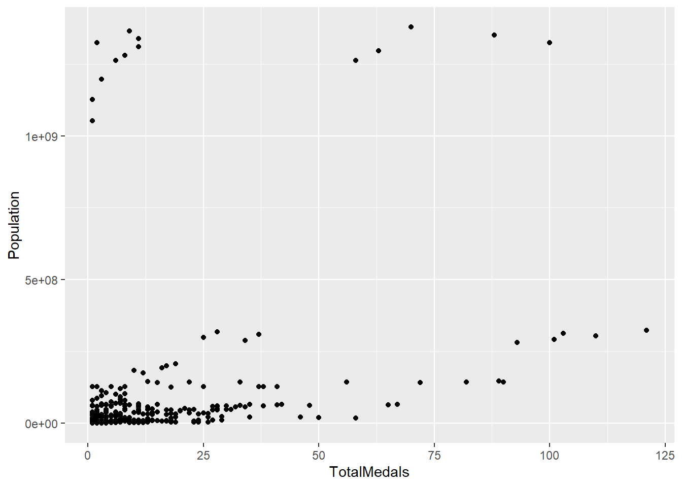
The results above indicate there may be a significant positive correlation between population size and medals won.
If we wanted to make the figure above a little bit more interactive we can do this using the plotly package (more on this in future sessions).
Last we will save the dataframes DatabyAthleteAvgDF, DatabyAthletePerYearDF, TotalsPerCountryYearDF and CountryDatawithPopDF as .RData as we will use them again in the next practical.
Exercise 8: Save the dataframes above as an .RData file named Practical5.RData.
Show the answer
save(DatabyAthleteAvgDF, DatabyAthletePerYearDF, TotalsPerCountryYearDF, CountryDatawithPopDF, file="C:/Users/wkb14101/OneDrive - University of Strathclyde/MSc SDA/R Projects/B1703/data/Practical5b.RData")