12  Practical 5a: Exploratory data analysis in R

During this demonstration we will recap conducting exploratory analysis in R. We will use the cleaned data files we used during the previous demonstration. If you want to follow along, the files can be found here.

First we will open the constructors, drivers, and race data.

Show the code

library(tidyverse)

ConstructorsDF<-read_rds("https://strath-my.sharepoint.com/:u:/g/personal/xanne_janssen_strath_ac_uk/Ea1fQLpdL4JImLeFNwn4ChkBBz2BJcEEBOhWYM5-m7bUHw?download=1")
DriversDF<-read_rds("https://strath-my.sharepoint.com/:u:/g/personal/xanne_janssen_strath_ac_uk/EVgCPbwNJKlAuG_hpBvxLpQBShiU1q16eWuRS19SFhj7VA?download=1")
RacesDF<-read_rds("https://strath-my.sharepoint.com/:u:/g/personal/xanne_janssen_strath_ac_uk/EaogXHpyrdVIm2bFiPiVpbQBl01YxYt9YHvunMfrCQzWiw?download=1")

12.1 Exploratory data analysis

Let’s first check the average age of the drivers. To do this we will need to create an age variable and make sure each drivers age is only taken into account once (remember each drivers has multiple row entries). As we want to obtain the age of the driver based on the race date we will need to conduct another merge of dataframes. So let’s start with merging the DriversDF with the RacesDF and calculating the age variable.

Show the code

# join the data using raceId as the unique identifier
DriversRacesDF <- merge(DriversDF, RacesDF, by= c("raceId"), all=TRUE)
#calculate age
DriversRacesDF <- DriversRacesDF %>%
      mutate(Age= time_length((date-dob),"years"))

Now we have the age of the drivers we can calculate the average age per year for each driver, and use this to create a line graph showcasing the change in F1 drivers from 1958 until 2024.

Show the code

#calculate average age by race year and driver (keep only one value for age per year/driver to avoid double counting)
DriversRacesDF <- DriversRacesDF %>%
  mutate(DriverName=paste(FirstName, LastName)) %>%
  group_by(RaceYear,driverId) %>%
  mutate(AverageAge = if_else(Age==max(Age,na.rm=TRUE),mean(Age, na.rm=TRUE), NA))

#create linegraph. Note how I use stat_summary, if you do not want to use stat_summary you would need to create a dataframe with the average age per year first (i.e. group_by(year))
LineGraphAge <- DriversRacesDF %>%
  distinct(driverId,AverageAge,.keep_all=TRUE) %>%
  filter(RaceYear>=1958)%>%
  ggplot(aes(RaceYear, AverageAge))+
  stat_summary(fun = mean, geom = "line", colour = "blue", size = 1)

LineGraphAge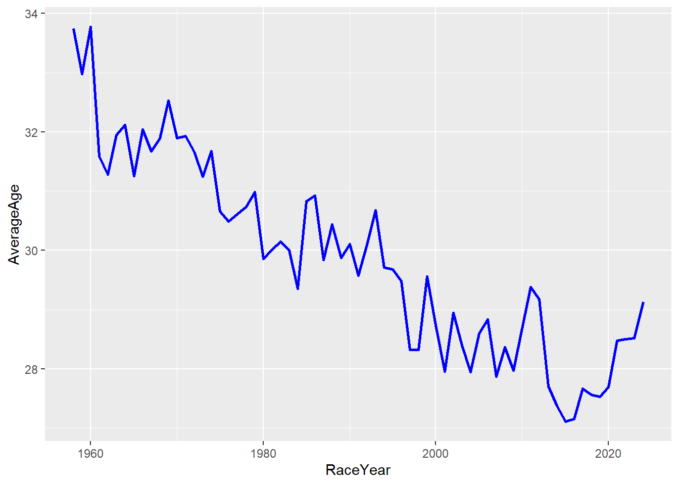

From the graph above we can see there has been a substantial decline in the average age of drivers in F1.

Next let’s look at how many different riders have won the championship, the average age when they won, as well as the youngest and oldest winners.

To do this we first need to identify the champions of each year. We will do this by looking at the their position at the end of the season. For this we need to find out how many rounds each year had, as we can then use that to assign the drivers an end of season position.

Show the code

# Get drivers position at end of the year
DriversRacesDF <- DriversRacesDF %>%
  group_by(RaceYear) %>%
  mutate(DriversFinalPosition = ifelse(RaceRound == max(RaceRound, na.rm = TRUE), DriversTotalPosition, NA))%>%
  ungroup()

library(flextable)

# Create summary stats for champions from 1958 onwards
SummaryStatsDF <- DriversRacesDF %>%
  filter(DriversFinalPosition == 1 & RaceYear >= 1958) %>%
  summarise(
    UniqueChampions = n_distinct(DriverName),
    Age_avg = mean(AverageAge, na.rm = TRUE),
    Age_min = min(AverageAge, na.rm = TRUE),
    Age_max = max(AverageAge, na.rm = TRUE),
    Wins_avg = mean(DriverWins, na.rm=TRUE),
    Wins_min = min(DriverWins, na.rm = TRUE),
    Wins_max = max(DriverWins, na.rm = TRUE)
  )

# Create a table in right shape for plotting
TableDF <- tibble(
  Variable = c("Unique Champions","Age (years)", "Wins"),
  Total = c(SummaryStatsDF$UniqueChampions, NA,NA),
  Average = c(NA,SummaryStatsDF$Age_avg, SummaryStatsDF$Wins_avg),
  Min = c(NA,SummaryStatsDF$Age_min, SummaryStatsDF$Wins_min),
  Max = c(NA,SummaryStatsDF$Age_max, SummaryStatsDF$Wins_max)
)

# Create the flextable
Table1 <- flextable(TableDF) %>%
  set_header_labels(
    Variable = "",
    Average = "Average",
    Min = "Minimum",
    Max = "Maximum") %>%
  theme_vanilla() %>%
  align(align = "center", part = "all") %>%
  valign(valign = "center", part = "header") %>% 
  autofit()

# Print the flextable
Table1

	Total	Average	Minimum	Maximum
Unique Champions	31
Age (years)		30.662744	23.03066	40.33463
Wins		6.590909	1.00000	19.00000

If I wanted to create a table with the average drivers age per year and standard deviation of age per year I would use a similar code as above, except I would group by RaceYear and not filter for just the winner (as that would give me only one entry per year which makes calculating an average and/or standard deviation redundant).

Show the code

TableDFPerYear<-DriversRacesDF %>%
  filter(RaceYear >= 1958) %>% #filter relevant years
  group_by(RaceYear)%>%
  reframe(UniqueDrivers= n_distinct(DriverName),
          Age_avg=mean(AverageAge, na.rm=TRUE),
          Age_std=sd(AverageAge, na.rm=TRUE),
          Age_min= min(AverageAge, na.rm=TRUE),
          Age_max= max(AverageAge, na.rm=TRUE),
          Wins_min= min(DriverWins, na.rm=TRUE),
          Wins_max= max(DriverWins, na.rm=TRUE))

flextable(TableDFPerYear) #Create basic Table

RaceYear	UniqueDrivers	Age_avg	Age_std	Age_min	Age_max	Wins_min	Wins_max
1,958	87	33.74429	6.379648	21.01643	58.95140	0	4
1,959	88	32.98062	5.916009	21.42460	46.48049	0	2
1,960	91	33.77181	6.067533	22.62955	47.47844	0	5
1,961	62	31.55727	6.203520	19.60849	48.52841	0	2
1,962	61	31.28101	6.152770	20.47669	52.49464	0	4
1,963	62	31.94821	6.831421	18.23135	53.44175	0	7
1,964	41	32.12268	6.613528	21.02204	47.62656	0	3
1,965	54	31.25979	5.197911	22.08038	44.58700	0	6
1,966	33	32.04609	4.227573	23.08517	40.33463	0	4
1,967	44	31.67535	5.961751	22.69624	45.93634	0	4
1,968	43	31.88735	5.332453	23.52704	46.88364	0	3
1,969	30	32.52852	6.329624	23.91513	47.89621	0	6
1,970	43	31.90064	5.473827	23.72856	45.60185	0	5
1,971	50	31.93036	5.076795	22.54689	46.58602	0	6
1,972	42	31.66242	4.821589	22.69131	47.58634	0	5
1,973	42	31.24877	4.337586	23.44274	44.42482	0	5
1,974	62	31.67150	4.266744	23.45225	45.32768	0	3
1,975	52	30.66415	3.984501	23.27845	46.29940	0	5
1,976	54	30.49249	3.245395	23.33949	38.63860	0	6
1,977	61	30.61654	4.017114	21.52374	39.61284	0	4
1,978	46	30.74011	4.909500	20.42659	40.73466	0	6
1,979	36	30.98851	4.763893	21.21725	41.87086	0	4
1,980	41	29.86114	5.526310	19.47502	42.85626	0	5
1,981	39	30.00795	4.825024	22.08661	41.33917	0	3
1,982	40	30.14940	5.017097	23.05014	42.34868	0	2
1,983	35	30.00776	4.336568	22.20744	39.59827	0	4
1,984	35	29.35463	4.038124	23.31902	40.61995	0	7
1,985	36	30.83146	4.513362	22.40840	41.67163	0	5
1,986	32	30.92709	4.653749	22.53936	42.63364	0	5
1,987	32	29.84104	3.777579	23.37183	39.09651	0	6
1,988	36	30.44227	4.314561	24.01215	40.07775	0	8
1,989	47	29.87936	4.180101	23.69952	41.05014	0	6
1,990	40	30.10647	4.192300	22.51677	37.92266	0	6
1,991	41	29.57319	4.449363	22.73192	38.91205	0	7
1,992	32	30.09895	4.330939	21.53572	38.91239	0	9
1,993	31	30.67537	5.522787	21.16222	39.26215	0	7
1,994	46	29.71650	4.507110	22.16359	41.07899	0	8
1,995	34	29.67954	4.675019	22.32535	42.00338	0	9
1,996	23	29.47950	4.569036	23.49918	38.55825	0	8
1,997	26	28.32388	4.596673	21.62811	37.86689	0	7
1,998	23	28.32605	4.176903	20.24978	37.78285	0	8
1,999	23	29.55745	4.081166	23.42368	38.86242	0	5
2,000	23	28.74339	4.181171	20.47091	36.11499	0	9
2,001	26	27.95307	4.568650	19.90079	37.03153	0	9
2,002	22	28.94406	4.702333	21.17882	36.61489	0	11
2,003	24	28.39765	4.189283	21.89733	36.85969	0	6
2,004	25	27.94991	4.441303	21.39493	37.82752	0	13
2,005	27	28.59809	3.846151	22.39706	36.49152	0	7
2,006	27	28.83353	4.532852	21.00662	37.48574	0	7
2,007	25	27.86791	4.483428	20.13216	36.35044	0	6
2,008	22	28.36342	4.646796	21.10609	37.31465	0	6
2,009	25	27.97156	5.196909	19.48905	38.66667	0	6
2,010	27	28.68005	5.352601	20.30923	41.52484	0	5
2,011	28	29.37744	5.718460	21.34313	42.55874	0	11
2,012	25	29.17600	5.528946	22.25955	43.56550	0	5
2,013	23	27.71162	4.205561	21.97846	36.91617	0	13
2,014	24	27.37823	4.241018	20.23473	34.75903	0	11
2,015	22	27.10912	4.942806	17.81692	35.77175	0	10
2,016	24	27.15609	5.155000	18.82181	36.77664	0	10
2,017	25	27.66884	5.505372	18.74483	37.77837	0	9
2,018	20	27.56199	5.397710	19.73899	38.77253	0	11
2,019	20	27.53091	5.615463	19.70340	39.77732	0	11
2,020	23	27.68901	5.178236	20.85646	40.93039	0	11
2,021	21	28.47606	6.387324	21.25344	41.82017	0	10
2,022	22	28.50541	5.320747	22.19513	40.97953	0	15
2,023	22	28.51844	5.624877	21.66516	41.99527	0	19
2,024	22	29.12940	6.002553	19.01661	42.77550	0	7

# Play around with specifications
          
TableFigPerYear <- flextable(TableDFPerYear) %>%
  colformat_double() %>%
  separate_header() %>%
  theme_vanilla() %>%
  align(align = "center", part = "all") %>%
  valign(valign = "center", part = "header") %>% 
  autofit()

TableFigPerYear

RaceYear	UniqueDrivers	Age				Wins
		avg	std	min	max	min	max
1,958	87	33.7	6.4	21.0	59.0	0	4
1,959	88	33.0	5.9	21.4	46.5	0	2
1,960	91	33.8	6.1	22.6	47.5	0	5
1,961	62	31.6	6.2	19.6	48.5	0	2
1,962	61	31.3	6.2	20.5	52.5	0	4
1,963	62	31.9	6.8	18.2	53.4	0	7
1,964	41	32.1	6.6	21.0	47.6	0	3
1,965	54	31.3	5.2	22.1	44.6	0	6
1,966	33	32.0	4.2	23.1	40.3	0	4
1,967	44	31.7	6.0	22.7	45.9	0	4
1,968	43	31.9	5.3	23.5	46.9	0	3
1,969	30	32.5	6.3	23.9	47.9	0	6
1,970	43	31.9	5.5	23.7	45.6	0	5
1,971	50	31.9	5.1	22.5	46.6	0	6
1,972	42	31.7	4.8	22.7	47.6	0	5
1,973	42	31.2	4.3	23.4	44.4	0	5
1,974	62	31.7	4.3	23.5	45.3	0	3
1,975	52	30.7	4.0	23.3	46.3	0	5
1,976	54	30.5	3.2	23.3	38.6	0	6
1,977	61	30.6	4.0	21.5	39.6	0	4
1,978	46	30.7	4.9	20.4	40.7	0	6
1,979	36	31.0	4.8	21.2	41.9	0	4
1,980	41	29.9	5.5	19.5	42.9	0	5
1,981	39	30.0	4.8	22.1	41.3	0	3
1,982	40	30.1	5.0	23.1	42.3	0	2
1,983	35	30.0	4.3	22.2	39.6	0	4
1,984	35	29.4	4.0	23.3	40.6	0	7
1,985	36	30.8	4.5	22.4	41.7	0	5
1,986	32	30.9	4.7	22.5	42.6	0	5
1,987	32	29.8	3.8	23.4	39.1	0	6
1,988	36	30.4	4.3	24.0	40.1	0	8
1,989	47	29.9	4.2	23.7	41.1	0	6
1,990	40	30.1	4.2	22.5	37.9	0	6
1,991	41	29.6	4.4	22.7	38.9	0	7
1,992	32	30.1	4.3	21.5	38.9	0	9
1,993	31	30.7	5.5	21.2	39.3	0	7
1,994	46	29.7	4.5	22.2	41.1	0	8
1,995	34	29.7	4.7	22.3	42.0	0	9
1,996	23	29.5	4.6	23.5	38.6	0	8
1,997	26	28.3	4.6	21.6	37.9	0	7
1,998	23	28.3	4.2	20.2	37.8	0	8
1,999	23	29.6	4.1	23.4	38.9	0	5
2,000	23	28.7	4.2	20.5	36.1	0	9
2,001	26	28.0	4.6	19.9	37.0	0	9
2,002	22	28.9	4.7	21.2	36.6	0	11
2,003	24	28.4	4.2	21.9	36.9	0	6
2,004	25	27.9	4.4	21.4	37.8	0	13
2,005	27	28.6	3.8	22.4	36.5	0	7
2,006	27	28.8	4.5	21.0	37.5	0	7
2,007	25	27.9	4.5	20.1	36.4	0	6
2,008	22	28.4	4.6	21.1	37.3	0	6
2,009	25	28.0	5.2	19.5	38.7	0	6
2,010	27	28.7	5.4	20.3	41.5	0	5
2,011	28	29.4	5.7	21.3	42.6	0	11
2,012	25	29.2	5.5	22.3	43.6	0	5
2,013	23	27.7	4.2	22.0	36.9	0	13
2,014	24	27.4	4.2	20.2	34.8	0	11
2,015	22	27.1	4.9	17.8	35.8	0	10
2,016	24	27.2	5.2	18.8	36.8	0	10
2,017	25	27.7	5.5	18.7	37.8	0	9
2,018	20	27.6	5.4	19.7	38.8	0	11
2,019	20	27.5	5.6	19.7	39.8	0	11
2,020	23	27.7	5.2	20.9	40.9	0	11
2,021	21	28.5	6.4	21.3	41.8	0	10
2,022	22	28.5	5.3	22.2	41.0	0	15
2,023	22	28.5	5.6	21.7	42.0	0	19
2,024	22	29.1	6.0	19.0	42.8	0	7

Next up let’s create a line chart of the winners age per year.

Show code

# create linegraph of the average age of the winners (note I could have used geom_line here instead of stat_summary as we only take one age per year)
LineGraphWinners <- DriversRacesDF %>%
  filter(DriversFinalPosition==1) %>%
  ggplot(aes(RaceYear, AverageAge)) +
  stat_summary(fun = mean, geom = "line", colour = "blue", size = 1)
  

LineGraphWinners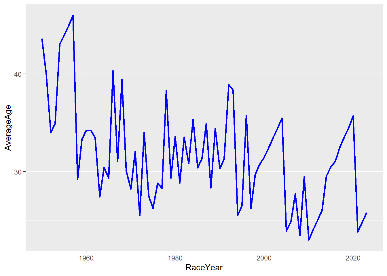

# Calculate max and min age of winners and annotate
MaxAge<- DriversRacesDF%>%
   filter(DriversFinalPosition==1) %>%
   slice_max(AverageAge)
  
MinAge<- DriversRacesDF%>%
   filter(DriversFinalPosition==1) %>%
   slice_min(AverageAge)

AnnotatedLineGraphWinners <- LineGraphWinners +
  geom_text(data=MaxAge,aes(label=DriverName),hjust=1.1, vjust=0.5)+
  geom_text(data=MinAge,aes(label=DriverName),hjust=1.1, vjust=0.5)+
  ylim(0,50)+
  labs(y="Champions Age", x="Year")

AnnotatedLineGraphWinners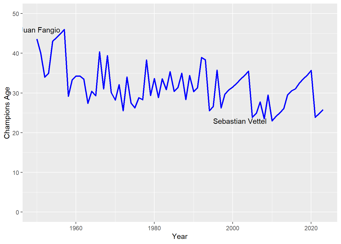

Lastly, we will look at the correlation between the fastest lap time per race and the average race time by creating a scatter plot.

Show the code

# summarise data for correlational plot (i.e. one data point per year per race)
CorData<-DriversRacesDF %>%
  filter(FastestLapTimeSec>=78) %>%
  group_by(RaceYear, raceId) %>%
  summarise(MinLapTime=min(FastestLapTimeSec, na.rm=TRUE),
            AvgRaceTime=mean(racetimeMin, na.rm=TRUE),
            GrandPrixName=unique(name)) %>%
  ungroup()

# create scatterplot
ScatterPlot<-ggplot(CorData, aes(AvgRaceTime,MinLapTime)) +
  geom_point()
ScatterPlot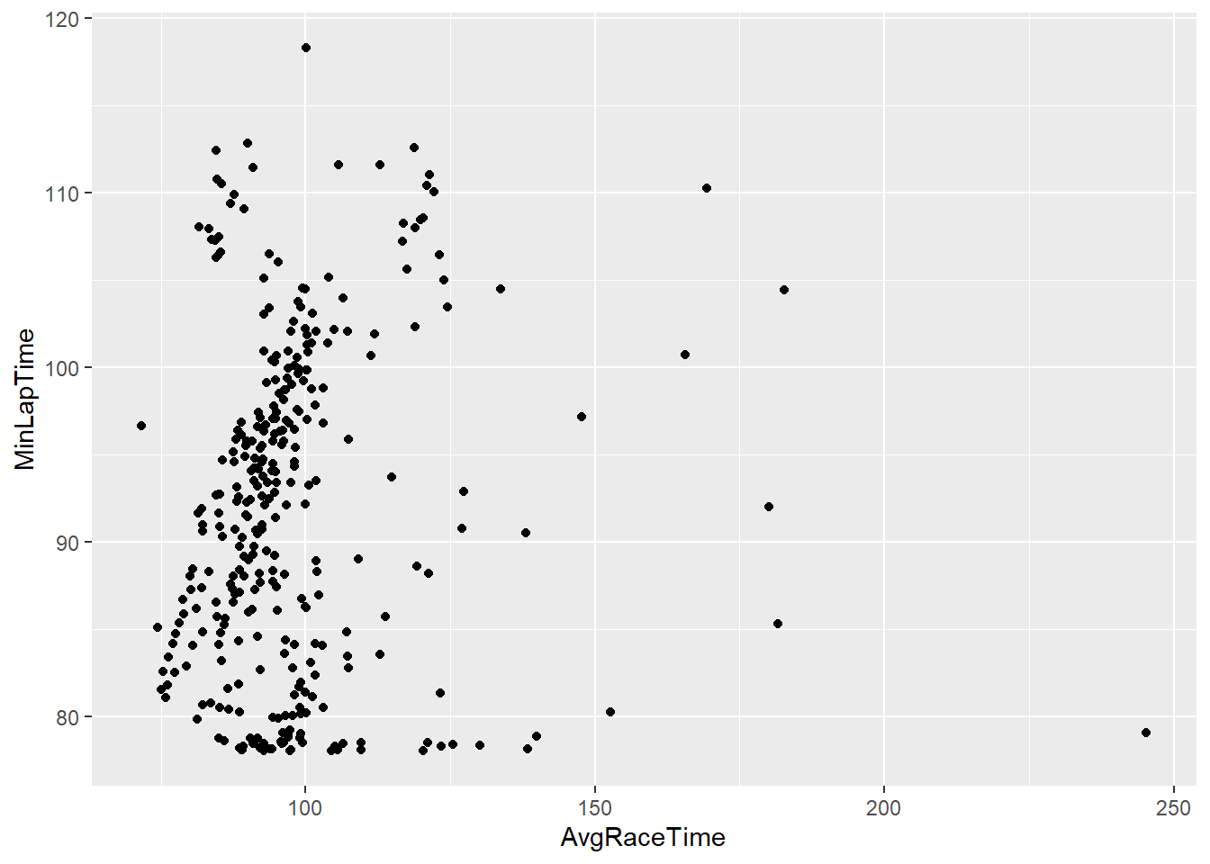

# identify max race time so we can check which grandprix this was
MaxRaceTime <- CorData%>%
  slice_max(AvgRaceTime)

# add annotations to highlight the longest race time grandprix
ScatterPlot<-ScatterPlot+
  geom_text(data=MaxRaceTime, aes(label=GrandPrixName), hjust=0.9, vjust=-1)+
  geom_text(data=MaxRaceTime, aes(label=RaceYear), hjust=2, vjust=1)

ScatterPlot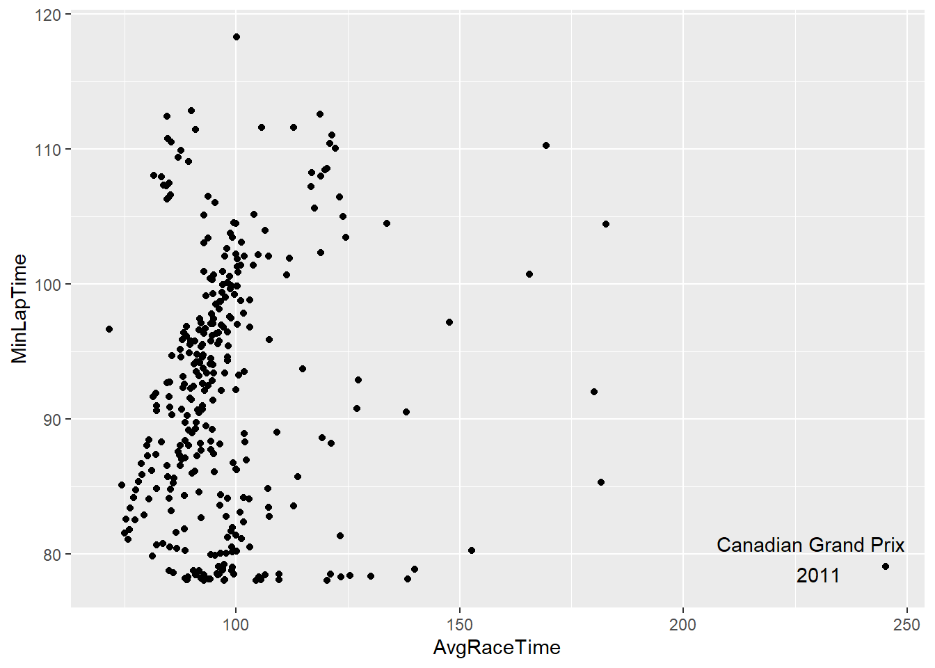

The scatterplot above shows on first view a weak correlation between the average race time and the fastest lap times. Point of interest is the high race time during the 2011 Canadian Grand Prix, worth looking into.

Last we will save the DriversDF, DriversRacesDF, ConstructorsDF, and RacesDF as an .RData file named Practical5_F1DriversRaces.RData.

Show the answer

save(DriversDF, DriversRacesDF, ConstructorsDF, ConstructorsDF,RacesDF, file="P5_F1Data.RData")
save.image(file="P5_F1.RData")