Show the code
#load required packages
rm(list=ls())
library(tidyverse)
library(corrplot)
library(fmsb)The objective of this practical is to guide you through the process of using data for recruitment purposes. It is crucial to note that before diving into data analysis, you should have already completed the necessary steps such as cleaning your data and identifying relevant KPIs. You should also ensure you understand how your data was collected. Analyzing data that is of unknown validity and reliability is not recommended. If you are unsure about the required steps, I recommend revisiting the previous sessions.
During this practical, you may encounter some unfamiliar code. However, there’s no need to worry too much about it. With more practice, the code will gradually become more understandable.
#load required packages
rm(list=ls())
library(tidyverse)
library(corrplot)
library(fmsb)In this practical we will use an NBA dataset. We will load this using:
# Set the filepath where the CSV file is located
#| code-fold: true
#| output: false
#| code-summary: "Show the answer"
#library openxlsx makes it easy to read xlsx files via shared links.
library(openxlsx)

# Set the filepath where the CSV file is located
FileDirectory <- "https://strath-my.sharepoint.com/:x:/g/personal/xanne_janssen_strath_ac_uk/EYxTNzBLTRZClpaT48ClGWIBtc-CmsGm2HvSOaX1uW05Rg?download=1"

NBADataDF <- read.xlsx(FileDirectory)The dataset you’ve been given is pretty clean but lets run a quick check to ensure all our data has been imported correctly before we start analysing some of the data.
#check structure

str(NBADataDF)
'data.frame': 812 obs. of 15 variables:
$ Rk : num 1 2 3 4 5 6 6 6 7 8 ...
$ Player : chr "Precious Achiuwa" "Steven Adams" "Bam Adebayo" "Santi Aldama" ...
$ Pos : chr "C" "C" "C" "PF" ...
$ Age : num 22 28 24 21 36 23 23 23 26 23 ...
$ Tm : chr "TOR" "MEM" "MIA" "MEM" ...
$ Games : num 73 76 56 32 47 65 50 15 66 56 ...
$ Minutes.Played : num 23.6 26.3 32.6 11.3 22.3 22.6 26.3 9.9 27.3 32.3 ...
$ Field.Goals : num 3.6 2.8 7.3 1.7 5.4 3.9 4.7 1.1 3.9 6.6 ...
$ Field.Goals.Attempted: num 8.3 5.1 13 4.1 9.7 10.5 12.6 3.2 8.6 9.7 ...
$ 3P : num 0.8 0 0 0.2 0.3 1.6 1.9 0.7 2.4 0 ...
$ 3P.attempted : num 2.1 0 0.1 1.5 1 5.2 6.1 2.2 5.9 0.2 ...
$ 2P : num 2.9 2.8 7.3 1.5 5.1 2.3 2.8 0.4 1.5 6.6 ...
$ 2P.attempted : num 6.1 5 12.9 2.6 8.8 5.3 6.5 1 2.7 9.6 ...
$ Free.Throws : num 1.1 1.4 4.6 0.6 1.9 1.2 1.4 0.7 1 2.9 ...
$ Free.Throws.Attempted: num 1.8 2.6 6.1 1 2.2 1.7 1.9 0.8 1.1 4.2 ...From the above we can see that Pos and Tm are character class. Let’s quickly change to factor. Also check for duplicates.
# Change Pos and Tm to factor
NBADataDF<- NBADataDF %>%
  mutate(Pos=as.factor(Pos),
         Tm=as.factor(Tm))

# First check if there are any players with more than one row
DuplicatedPlayers<-NBADataDF$Player[duplicated(NBADataDF$Player)]
unique(DuplicatedPlayers)
[1] "Nickeil Alexander-Walker" "Justin Anderson"
[3] "D.J. Augustin" "Marvin Bagley III"
[5] "DeAndre' Bembry" "DÄ\u0081vis BertÄ\u0081ns"
[7] "Armoni Brooks" "Charlie Brown Jr."
[9] "Chaundee Brown Jr." "Moses Brown"
[11] "Vernon Carey Jr." "Jevon Carter"
[13] "Willie Cauley-Stein" "DeMarcus Cousins"
[15] "Robert Covington" "Torrey Craig"
[17] "Seth Curry" "Spencer Dinwiddie"
[19] "Donte DiVincenzo" "Jeff Dowtin"
[21] "Goran Dragić" "Andre Drummond"
[23] "James Ennis III" "Drew Eubanks"
[25] "Bruno Fernando" "Malik Fitts"
[27] "Bryn Forbes" "Tim Frazier"
[29] "Wenyen Gabriel" "Langston Galloway"
[31] "Tyrese Haliburton" "James Harden"
[33] "Montrezl Harrell" "Josh Hart"
[35] "Juancho Hernangómez" "Buddy Hield"
[37] "Malcolm Hill" "Aaron Holiday"
[39] "Justin Holiday" "Rodney Hood"
[41] "Danuel House Jr." "Elijah Hughes"
[43] "Serge Ibaka" "Josh Jackson"
[45] "Justin Jackson" "Alize Johnson"
[47] "Keon Johnson" "Tyler Johnson"
[49] "Carlik Jones" "DeAndre Jordan"
[51] "Georgios Kalaitzakis" "Braxton Key"
[53] "Kevin Knox" "Luke Kornet"
[55] "Jeremy Lamb" "Romeo Langford"
[57] "Caris LeVert" "Didi Louzada"
[59] "Trey Lyles" "Kelan Martin"
[61] "Mac McClung" "CJ McCollum"
[63] "Paul Millsap" "Greg Monroe"
[65] "Juwan Morgan" "Mychal Mulder"
[67] "Larry Nance Jr." "Semi Ojeleye"
[69] "Reggie Perry" "Kristaps Porziņģis"
[71] "Norman Powell" "Cam Reddish"
[73] "Josh Richardson" "Justin Robinson"
[75] "Rajon Rondo" "Domantas Sabonis"
[77] "Tomáš Satoranský" "Dennis Schröder"
[79] "Chris Silva" "Javonte Smart"
[81] "Ish Smith" "Jalen Smith"
[83] "Xavier Sneed" "Tony Snell"
[85] "Nik Stauskas" "Lance Stephenson"
[87] "Daniel Theis" "Isaiah Thomas"
[89] "Tristan Thompson" "Rayjon Tucker"
[91] "Denzel Valentine" "Brad Wanamaker"
[93] "Tremont Waters" "Derrick White"
[95] "Justise Winslow" "Moses Wright"
[97] "Thaddeus Young" Now we have loaded in and cleaned our data it is time to start our analysis.
First we want to check if any variables correlate with minutes played (we expect those who have played more will have more opportunities to score). If we find a high correlation, ensure you create variables which correct for this.
#  Check correlation
Correlation<- cor(NBADataDF[,c(6:14)],use="complete.obs")
Correlation
Games Minutes.Played Field.Goals
Games 1.0000000 0.6202829 0.5639869
Minutes.Played 0.6202829 1.0000000 0.8869035
Field.Goals 0.5639869 0.8869035 1.0000000
Field.Goals.Attempted 0.5424375 0.8986102 0.9708558
3P 0.4759508 0.7204720 0.6791450
3P.attempted 0.4577036 0.7326663 0.6801109
2P 0.4842288 0.7735922 0.9360769
2P.attempted 0.4734385 0.8030827 0.9445314
Free.Throws 0.4051912 0.6966496 0.8208116
Field.Goals.Attempted 3P 3P.attempted 2P
Games 0.5424375 0.4759508 0.4577036 0.4842288
Minutes.Played 0.8986102 0.7204720 0.7326663 0.7735922
Field.Goals 0.9708558 0.6791450 0.6801109 0.9360769
Field.Goals.Attempted 1.0000000 0.7648605 0.7944972 0.8584772
3P 0.7648605 1.0000000 0.9698270 0.3781567
3P.attempted 0.7944972 0.9698270 1.0000000 0.3935001
2P 0.8584772 0.3781567 0.3935001 1.0000000
2P.attempted 0.9079288 0.4444589 0.4669812 0.9787224
Free.Throws 0.7980833 0.4782479 0.4898463 0.8064177
2P.attempted Free.Throws
Games 0.4734385 0.4051912
Minutes.Played 0.8030827 0.6966496
Field.Goals 0.9445314 0.8208116
Field.Goals.Attempted 0.9079288 0.7980833
3P 0.4444589 0.4782479
3P.attempted 0.4669812 0.4898463
2P 0.9787224 0.8064177
2P.attempted 1.0000000 0.8245790
Free.Throws 0.8245790 1.0000000#High correlation between minutes played and on field actions. We will correct for minutes played and create a variable per 48 minutes (basketball match lasts 48 minutes).
NBADataDF<- NBADataDF%>%
mutate(across(c(Field.Goals, Field.Goals.Attempted, `3P`,`3P.attempted`,`2P`, `2P.attempted`, Free.Throws, Free.Throws.Attempted), ~(.x/Minutes.Played)*48, .names = "Per48_{.col}"))
#Check correlation - reduced
Correlation<- cor(NBADataDF[,c(7,16:22)],use="complete.obs")
Correlation Minutes.Played Per48_Field.Goals
Minutes.Played 1.0000000 0.41053662
Per48_Field.Goals 0.4105366 1.00000000
Per48_Field.Goals.Attempted 0.3458232 0.70344436
Per48_3P 0.3647455 0.22389443
Per48_3P.attempted 0.1628142 0.04919852
Per48_2P 0.2397172 0.89404818
Per48_2P.attempted 0.2390579 0.73395679
Per48_Free.Throws 0.2178295 0.28916729
Per48_Field.Goals.Attempted Per48_3P
Minutes.Played 0.3458232 0.364745462
Per48_Field.Goals 0.7034444 0.223894433
Per48_Field.Goals.Attempted 1.0000000 0.401523682
Per48_3P 0.4015237 1.000000000
Per48_3P.attempted 0.5085698 0.797457011
Per48_2P 0.5177669 -0.233643812
Per48_2P.attempted 0.6605479 -0.251466087
Per48_Free.Throws 0.3327476 -0.003876764
Per48_3P.attempted Per48_2P Per48_2P.attempted
Minutes.Played 0.16281419 0.2397172 0.2390579
Per48_Field.Goals 0.04919852 0.8940482 0.7339568
Per48_Field.Goals.Attempted 0.50856984 0.5177669 0.6605479
Per48_3P 0.79745701 -0.2336438 -0.2514661
Per48_3P.attempted 1.00000000 -0.3163942 -0.3093328
Per48_2P -0.31639417 1.0000000 0.8474461
Per48_2P.attempted -0.30933283 0.8474461 1.0000000
Per48_Free.Throws -0.07872921 0.2887601 0.4378172
Per48_Free.Throws
Minutes.Played 0.217829494
Per48_Field.Goals 0.289167290
Per48_Field.Goals.Attempted 0.332747563
Per48_3P -0.003876764
Per48_3P.attempted -0.078729215
Per48_2P 0.288760067
Per48_2P.attempted 0.437817200
Per48_Free.Throws 1.000000000When comparing KPIs it would be easier to have an overview of a players total number of games and average numbers of goals etc for each of the measures. We can create a new table with one row per athlete using group_by() and summarize() functions
# create a summary score so each player has one row (note how I summed the total games but took averages for the rest in line the variables). Duplicate rows are removed at the end
NBADataSummaryDF <- NBADataDF %>%
  group_by(Player) %>%
  summarise(Games = sum(Games),
            Pos = Pos,
            across(where(is.numeric), mean,.names="{.col}")) %>%
  distinct(Player, .keep_all = TRUE) %>%
ungroup()Now let’s look at the top performing players based on highest percentage of successful field goals.
NBADataSummaryDF <- NBADataSummaryDF %>%
  mutate(PerFieldGoals = (Per48_Field.Goals/Per48_Field.Goals.Attempted)*100)

NBADataSummaryDF %>%
  arrange(desc(PerFieldGoals)) %>%
  head(10)
# A tibble: 10 × 23
Player Games Pos Rk Age Minutes.Played Field.Goals
<chr> <dbl> <fct> <dbl> <dbl> <dbl> <dbl>
1 Ahmad Caver 1 SG 99 25 1 1
2 Jaden Springer 2 SG 515 19 3 0.5
3 Joe Johnson 1 SG 285 40 2 1
4 Tyrell Terry 2 PG 530 21 1.5 0.5
5 Ed Davis 31 C 128 32 6.5 0.4
6 Jericho Sims 41 PF 506 23 13.5 1
7 Craig Sword 3 SG 523 28 6.3 1
8 Udoka Azubuike 17 C 23 22 11.5 2.2
9 Mitchell Robinson 72 C 478 23 25.7 3.6
10 D.J. Wilson 4 PF 591 25 13.5 2.8
# ℹ 16 more variables: Field.Goals.Attempted <dbl>, `3P` <dbl>,
# `3P.attempted` <dbl>, `2P` <dbl>, `2P.attempted` <dbl>, Free.Throws <dbl>,
# Free.Throws.Attempted <dbl>, Per48_Field.Goals <dbl>,
# Per48_Field.Goals.Attempted <dbl>, Per48_3P <dbl>,
# Per48_3P.attempted <dbl>, Per48_2P <dbl>, Per48_2P.attempted <dbl>,
# Per48_Free.Throws <dbl>, Per48_Free.Throws.Attempted <dbl>,
# PerFieldGoals <dbl>You may have seen from the above that the top 40 played less than 5 minutes and attempted less than 1 field goal on average. To obtain a fairer top 10 we need to filter for minutes played and potentially if you want for field goals attempted. We will focus on those playing more than 10 minutes on average.
# First we wil create a new data table showing the players with the top 10 runs, making sure only those with a minimum of 10 minutes are included.
Top10PerFieldGoalsDF<-NBADataSummaryDF %>%
  filter(Minutes.Played>10)%>%
  arrange(desc(PerFieldGoals)) %>%
  slice(1:10)


# Next we use ggplot to plot a bar chart of those recording the top 10

Figure1<-ggplot(Top10PerFieldGoalsDF, aes(reorder(Player,-PerFieldGoals),
                              y=PerFieldGoals)) + geom_col(show.legend = FALSE) + ggtitle("Top 10 Field Goals")+
  geom_text(aes(label = round(PerFieldGoals,1), vjust = -0.1))+theme(axis.text.x = element_text(angle = 60, hjust = 1),
        plot.title = element_text(hjust=0.5, colour="Black",
size=20)) + labs(y="% Goals Scored", x= "Player")Now we have the top 10 for our main KPI Percentage Field Goals we can compare the number 1 and number 10 based on PerFieldGoals, Per48_Free.Throws, Per48_3P, and Per48_2P.
# First we need to define the columns to normalize as we want all values to range between 0-1. We will normalise our KPIs
ColumnsToNormalize <- c("PerFieldGoals", "Per48_Free.Throws", "Per48_3P", "Per48_2P")

# Compute the maximum values for the specified columns. To normalise to 1 we will need to know the max value present for each variable in the full dataset, this will be listed in a vector called max_values.

NBADataSummaryFilteredDF <- NBADataSummaryDF %>%
  filter(Minutes.Played>10)

MaxValues <- apply(NBADataSummaryFilteredDF[,ColumnsToNormalize], 2, max,na.rm=TRUE)

# Normalize the specified columns (column values / MaxValues)
NormalizedColumnsDF <- sweep(NBADataSummaryFilteredDF[, ColumnsToNormalize], 2, MaxValues, "/")
colnames(NormalizedColumnsDF) <- paste('Norm', colnames(NormalizedColumnsDF), sep = '_')


# Add the normalized columns back to the filtered data frame
NBADataSummaryFilteredDF <- cbind(NBADataSummaryFilteredDF, NormalizedColumnsDF)

# Filter for specific athletes (here we filter for top 5 batting strike rate)
Top10PerFieldGoals <- NBADataSummaryFilteredDF %>%
  arrange(desc(PerFieldGoals)) %>%
  slice(1:10)

#select the data for the radar chart
RadarDataDF <- Top10PerFieldGoals[c(1,10),c("Norm_PerFieldGoals", "Norm_Per48_Free.Throws", "Norm_Per48_3P", "Norm_Per48_2P", "Player")]


RadarDataDF <- data.frame(PerFieldGoals = c(1, 0, RadarDataDF$Norm_PerFieldGoals),
Per48_Free.Throws = c(1, 0, RadarDataDF$Norm_Per48_Free.Throws),
Per48_3P = c(1, 0, RadarDataDF$Norm_Per48_3P),
Per48_2P = c(1, 0, RadarDataDF$Norm_Per48_2P),
row.names=c("max","min",RadarDataDF$Player))

# Create the radar chart
RadarPlot <- radarchart(
  RadarDataDF,axistype=0,vlabels=c("FG","FT", "3P","2P"), centerzero=TRUE, pcol= c("#00AFBB", "#E7B800"))

legend(x="topleft" , legend = rownames(RadarDataDF[-c(1,2),]), horiz = FALSE, bty = "n", pch=20, col=c("#00AFBB", "#E7B800"), cex=1, pt.cex=1.5)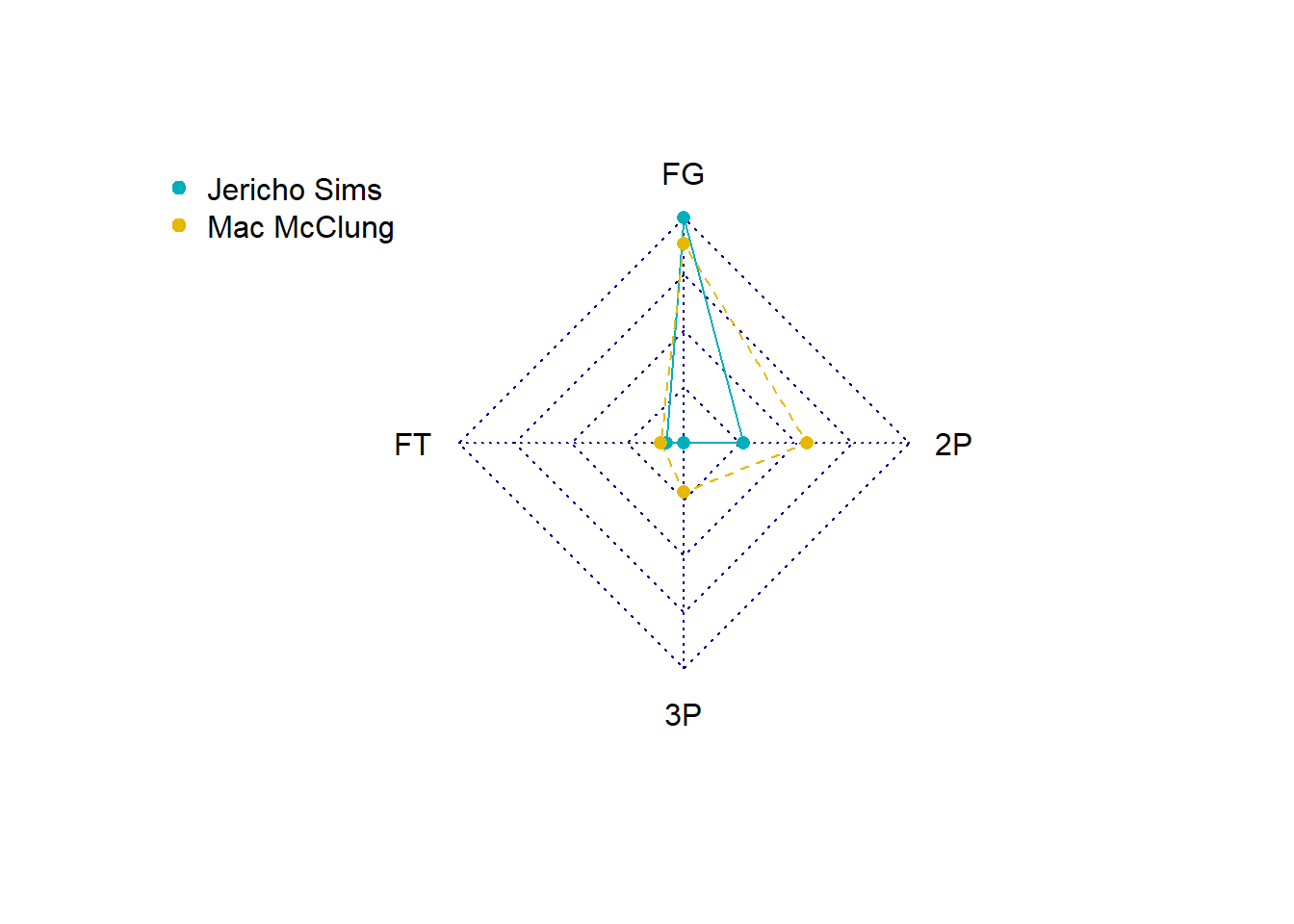
# Print the radar chart
print(RadarPlot)NULLFrom these tables we can see that the top 10 players differ per KPI. It is therefore important to have an understanding about which KPIs are most valuable. Another option would be to create a composite score which includes all KPIs based on specific weightings. We will look at that next week.