Show the code
knitr::opts_chunk$set(warning = FALSE, message = FALSE)
rm(list=ls())
library(tidyverse)
library(corrplot)
library(fmsb)
library(summarytools)
library(moments)
library(caret)During your case study you developed a talent identification program and identified relevant KPIs for talented cyclists. During this practical we will use the knowledge gained during your practical case study and work with a dataset which includes data on 1000 cyclist to identify the top performing male cyclists age 15-17y. We have the following data:
| Date of birth | Lactate threshold |
| Gender | Peak power output |
| Height | Technical skill ability |
| Weight | Beck anxiety score |
| Years of experience competing | GSE self-efficacy score |
| VO2max | Attention score |
For this practical we will use a variety of packages. It is important you install and start tidyverse, corrplot, fmsb, summarytools, moments, and caret.
knitr::opts_chunk$set(warning = FALSE, message = FALSE)
rm(list=ls())
library(tidyverse)
library(corrplot)
library(fmsb)
library(summarytools)
library(moments)
library(caret)Once you have successfully installed and loaded all the necessary packages, you can load in your data. We will load in CyclingTI.csv and assign it to CyclingDataDF. The data can be found on myplace but can also be loaded using the following shared link:
# Set the directory where the CSV files are located
file_path <- "https://strath-my.sharepoint.com/:x:/g/personal/xanne_janssen_strath_ac_uk/ESWr_kmjIRtIu-5RxgMdzpIBGbBd4jc4nH4wbNXGmmNKeg?download=1"

CyclingDataDF <- as_tibble(read.csv(file_path))Throughout the practicals you will note I often use “as_tibble()”. Tibbles are data frames, but they display data in a condensed format so it does not overwhelm your screen. Tibbles are also more strict when it comes to input: they never partial match a variable name, and they will generate a warning if the column you are trying to access does not exist.
Once we open the data we need to make sure we understand the meaning of all variables. A data dictionary can be found here.
At a first glance our data looks fairly structured and clean but we will do a few quick checks to make sure there are no obvious errors (see Practical 2 for more detailed description of cleaning data in R). We start by checking the structure.
# Check the structure of the data
str(CyclingDataDF)
tibble [1,000 × 17] (S3: tbl_df/tbl/data.frame)
$ Cyclist_ID : int [1:1000] 999 812 717 797 933 724 657 667 859 996 ...
$ Date_of_Birth : chr [1:1000] "13/08/2007" "16/04/2008" "27/10/2011" "14/02/2006" ...
$ Gender : chr [1:1000] "Female" "Female" "Female" "Female" ...
$ Age : int [1:1000] 15 15 11 17 14 12 16 12 15 16 ...
$ ftp : num [1:1000] 149 185 215 189 185 ...
$ anxiety : int [1:1000] 1 14 16 10 2 11 2 11 11 5 ...
$ vo2_max : num [1:1000] 72 57.2 53.4 62.5 82.1 ...
$ lactate_threshold: num [1:1000] 203 207 219 219 227 ...
$ peak_power : num [1:1000] 234 202 223 212 238 ...
$ weight : num [1:1000] 40.8 43.9 44.3 44.6 44.7 ...
$ height : num [1:1000] 136 137 139 142 142 ...
$ years_experience : int [1:1000] 6 3 3 5 5 10 1 5 1 1 ...
$ technical_skill : int [1:1000] 9 10 3 5 8 7 9 2 6 2 ...
$ self_efficacy : int [1:1000] 13 32 13 40 18 18 37 34 14 38 ...
$ attention : int [1:1000] 58 67 57 76 50 93 58 48 81 67 ...
$ wins_national : int [1:1000] 17 10 10 11 2 18 8 0 1 2 ...
$ wins_regional : int [1:1000] 4 0 0 25 20 22 12 5 15 8 ...Looking at the output above we can see that all numerical variables have been assigned the integer data type, the only variable for which a change of data type is required is Date_of_Birth. This is currently a character data type but should be date.
# Change date of birth to date
CyclingDataDF <- CyclingDataDF %>%
      mutate(Date_of_Birth = dmy(Date_of_Birth))
Next we will quickly check for any missing variables. We already know there are no empty variables so we will just check for any missing row data.
# Screen for missing row data
cat("Total missing data:","\n", sum(is.na(CyclingDataDF)), "\n")
Total missing data:
0 cat("\n","Missing data per variable:","\n")
Missing data per variable: print(colSums(is.na(CyclingDataDF))) Cyclist_ID Date_of_Birth Gender Age
0 0 0 0
ftp anxiety vo2_max lactate_threshold
0 0 0 0
peak_power weight height years_experience
0 0 0 0
technical_skill self_efficacy attention wins_national
0 0 0 0
wins_regional
0 The output above shows us that we have a full set of data without any missing data. Let’s check if there are any duplicates.
# Check for duplicates
which(duplicated(CyclingDataDF))integer(0)No duplicates were identified. Before we check for outliers and obtain some summary statistics we will want to filter our dataset to only include those of interest to us. For this analysis, we are only interested in males between 15-17 years of age so let’s filter for this.
# Remove duplicates
CyclingDataFilteredDF <- CyclingDataDF %>%
  filter(Gender == "Male" & Age >= 15 & Age <= 17)
After filtering we have 207 cyclists who fit our criteria, we can now start looking at our data.
The first thing we want to do is check the distribution of our data and check for outliers and errors in the data. Let’s calculate the summary statistics for each numerical variable and print them.
# Check for errors and outliers in each numerical variable
NumericVarsDF <- CyclingDataFilteredDF %>%
  select_if(is.numeric)

for (var in names(NumericVarsDF)) {
  var_summary <- summary(NumericVarsDF[[var]],na.rm=TRUE)

  # Print summary statistics
  cat("Variable:", var, "\n")
  print(var_summary)
  cat("\n")
  }
Variable: Cyclist_ID
Min. 1st Qu. Median Mean 3rd Qu. Max.
1.0 168.0 314.0 306.7 455.0 591.0
Variable: Age
Min. 1st Qu. Median Mean 3rd Qu. Max.
15.00 15.00 16.00 15.79 16.00 17.00
Variable: ftp
Min. 1st Qu. Median Mean 3rd Qu. Max.
166.0 221.2 270.8 276.4 321.9 461.6
Variable: anxiety
Min. 1st Qu. Median Mean 3rd Qu. Max.
0.000 5.000 10.000 9.739 15.000 20.000
Variable: vo2_max
Min. 1st Qu. Median Mean 3rd Qu. Max.
23.98 52.53 60.53 59.72 67.34 87.24
Variable: lactate_threshold
Min. 1st Qu. Median Mean 3rd Qu. Max.
50.23 283.24 304.07 300.29 319.75 379.01
Variable: peak_power
Min. 1st Qu. Median Mean 3rd Qu. Max.
250.8 379.8 462.4 465.5 539.0 761.6
Variable: weight
Min. 1st Qu. Median Mean 3rd Qu. Max.
48.21 55.22 59.73 61.29 67.23 88.69
Variable: height
Min. 1st Qu. Median Mean 3rd Qu. Max.
132.3 158.4 167.7 169.1 176.4 218.5
Variable: years_experience
Min. 1st Qu. Median Mean 3rd Qu. Max.
1.000 3.000 5.000 5.425 8.000 10.000
Variable: technical_skill
Min. 1st Qu. Median Mean 3rd Qu. Max.
1.000 3.000 6.000 5.556 8.000 10.000
Variable: self_efficacy
Min. 1st Qu. Median Mean 3rd Qu. Max.
10.00 17.00 26.00 25.28 33.00 40.00
Variable: attention
Min. 1st Qu. Median Mean 3rd Qu. Max.
30.00 46.00 66.00 65.23 81.00 100.00
Variable: wins_national
Min. 1st Qu. Median Mean 3rd Qu. Max.
0.00 4.00 8.00 8.43 12.00 20.00
Variable: wins_regional
Min. 1st Qu. Median Mean 3rd Qu. Max.
0.00 7.00 13.00 13.55 20.00 30.00 Looking at the summary statistics there are a few things to note, VO2max includes a minimum of 23.9794108. A VO2max below 32 is normally only seen in very unfit people or those with a medical condition. Given all these athletes are cyclist we can assume there has been either a data entry error or a measurement fault. Similar there are some very low and high values for lactate threshold (min: 50.23 and max: 379.01), these could be erroneous and should be evaluated with care (e.g. if an athlete has a high FTP it is very likely the low lactate threshold value is an error) and in this situation I will apply some minimum values required to be included in the analysis. I would expect the VO2max to be above 40 and the lactate threshold to be above 100. If my values are below this I will replace them with NA. Note I do not delete all of the athletes data as it could be just one data entry error for that variable and the other data may still be useful.
CyclingDataFilteredDF$lactate_threshold <- ifelse(CyclingDataFilteredDF$lactate_threshold<100,NA,CyclingDataFilteredDF$lactate_threshold)
CyclingDataFilteredDF$vo2_max <- ifelse(CyclingDataFilteredDF$vo2_max<40,NA,CyclingDataFilteredDF$vo2_max)
# Making sure the numeric vars variable is up to date.
NumericVarsDF <- CyclingDataFilteredDF %>%
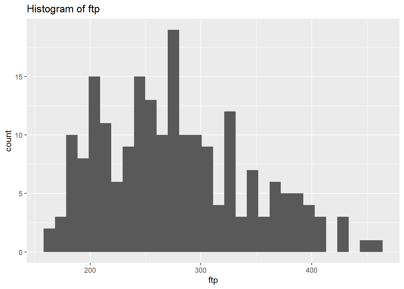
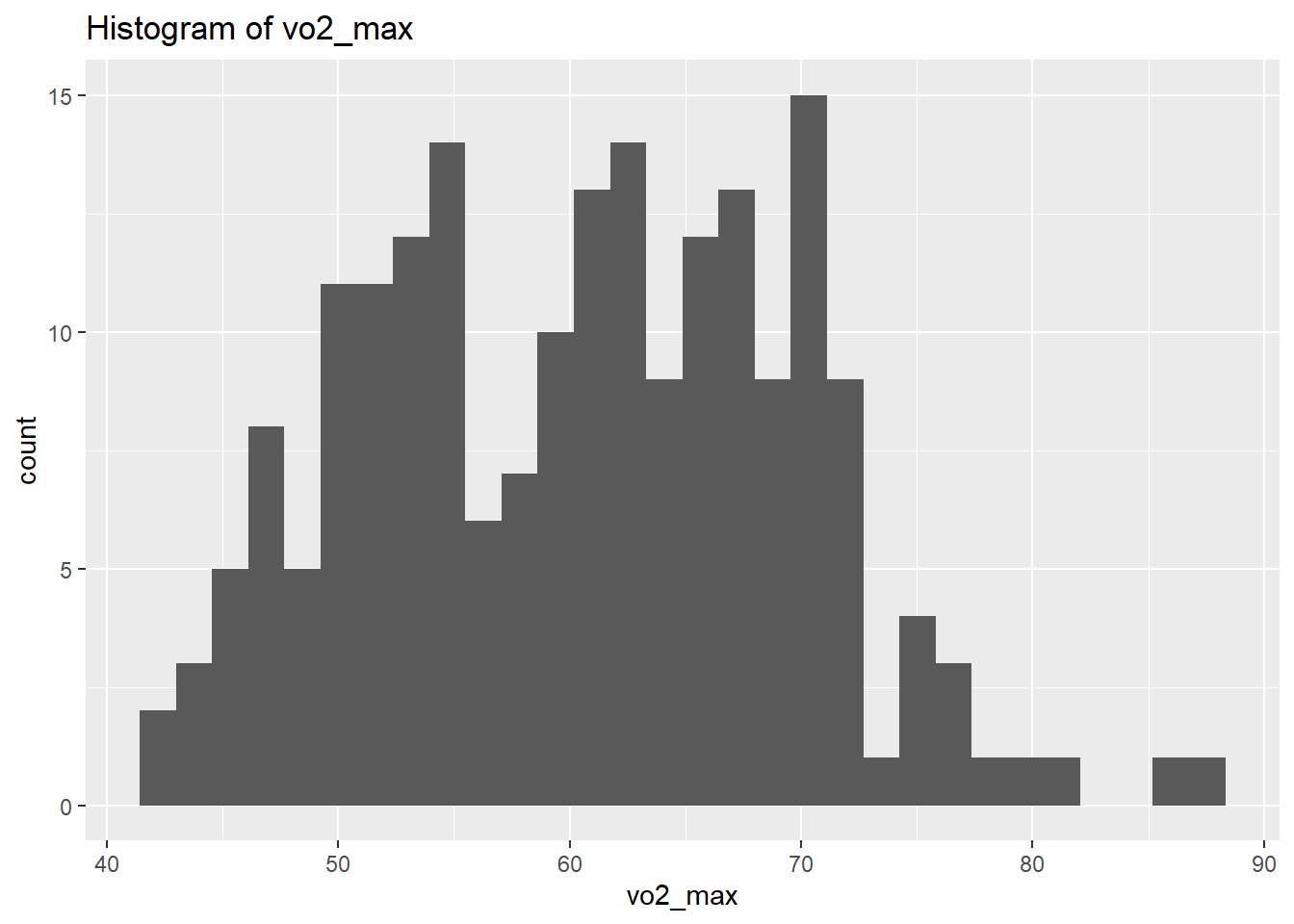
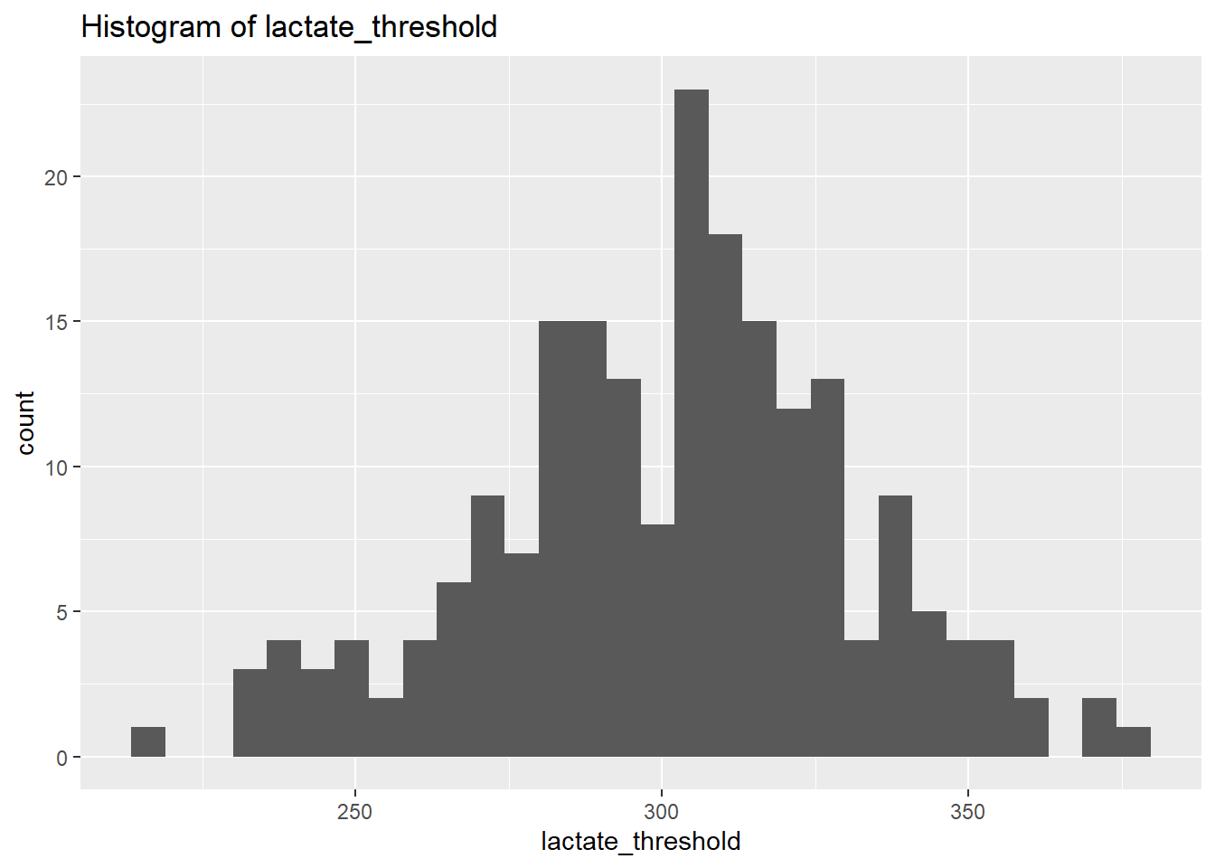
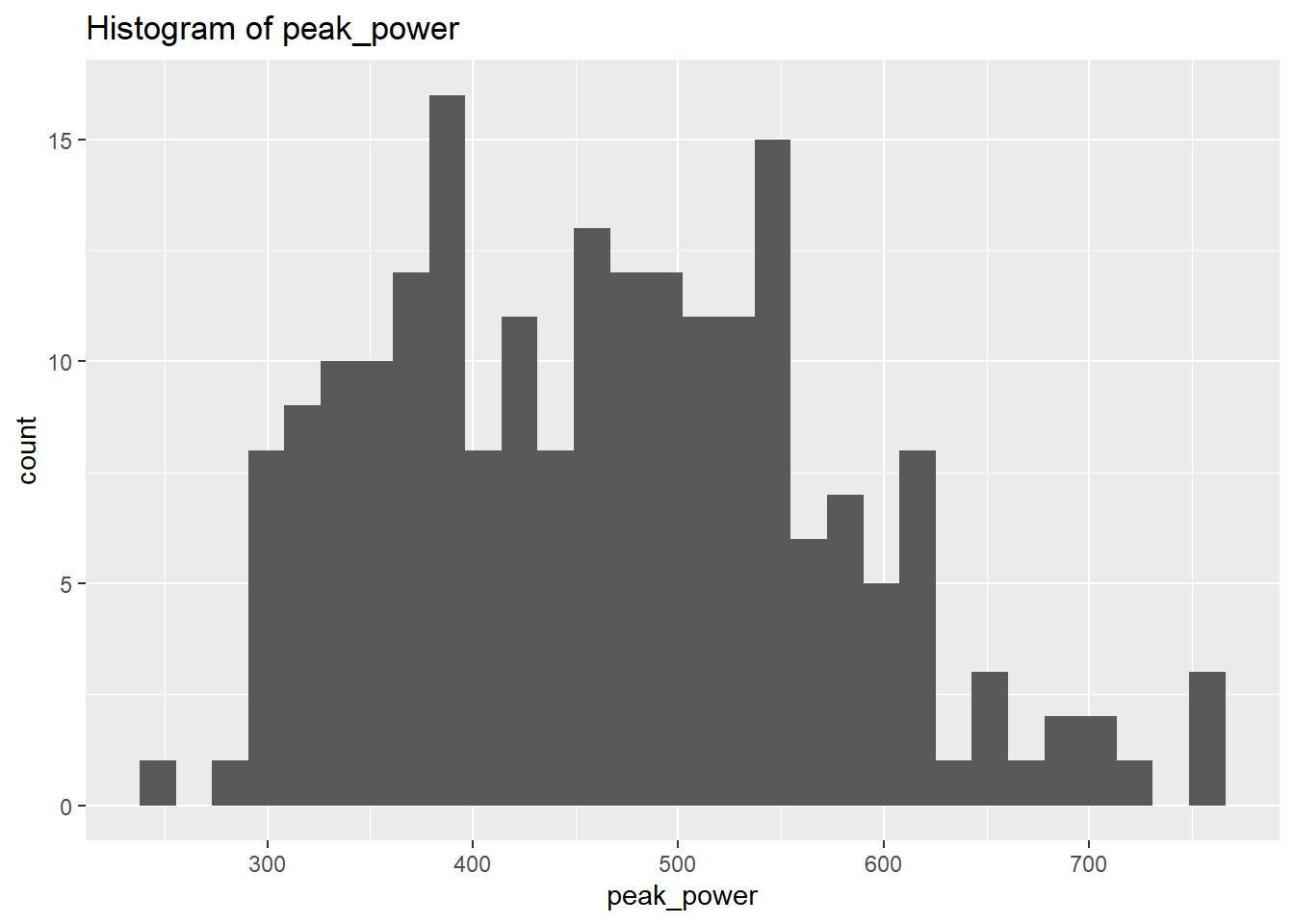
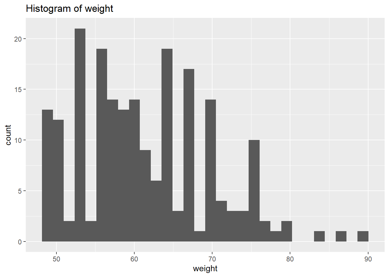
select_if(is.numeric)We will use plots in order to visualise the distribution of the data. However, instead of focusing on all let’s focus on the outputs we’re interested in for now. Let’s select the physiological outcomes of ftp, VO2max, lactate threshold, peak power and weight.
# Create a histogram to visualize the distribution and outliers of our numerical data

NumericVarsDF<-NumericVarsDF %>%
  select(3,5:8)

for (var in names(NumericVarsDF)) {
    histo<-ggplot(data = CyclingDataFilteredDF, aes_string(var)) +
      geom_histogram() +
      ggtitle(paste("Histogram of", var))
    print(histo)
}
for (var in names(NumericVarsDF)) {
  cat(var, "Skewness:", skewness(CyclingDataFilteredDF[[var]],na.rm = TRUE),"\n")
  cat(var, "Kurtosis:",kurtosis(CyclingDataFilteredDF[[var]],na.rm=TRUE),"\n")
  }
ftp Skewness: 0.5132121
ftp Kurtosis: 2.562371
vo2_max Skewness: 0.1390955
vo2_max Kurtosis: 2.478389
lactate_threshold Skewness: -0.1953618
lactate_threshold Kurtosis: 3.001187
peak_power Skewness: 0.4109461
peak_power Kurtosis: 2.664983
weight Skewness: 0.5661626
weight Kurtosis: 2.857294 From the above we can see that based on the skewness and kurtosis values, the majority of continues variables are relatively normally distributed (they are not all perfect and depending on future analysis we may need to transform them but for now we will leave them as they are).
Skewness a measure of the asymmetry of the distribution. A distribution can be skewed to the left (negative) or right (positive). A skewness of 0 means an equal distribution to either side.
Kurtosis is a measure of the tailedness of a distribution. Distributions can have medium tails (normal distribution resulting in a excess kurtosis of 0), thin tails (resulting in a negative excess kurtosis), and fat tails (resulting in a positive excess kurtosis).
Now let’s start with some simple analysis. First we want to explore if any of our physiological measures may be correlated with weight or age. If this is the case we may want to think about creating variables that can correct for this (e.g. we know that power output is heavily influenced by the size of an athlete).
CorrelationMatrix <-cor(NumericVarsDF,use="complete.obs")
CorrelationMatrix
ftp vo2_max lactate_threshold peak_power weight
ftp 1.00000000 0.03609121 0.10863184 0.30847039 0.58733982
vo2_max 0.03609121 1.00000000 0.05697213 0.05133952 0.01689525
lactate_threshold 0.10863184 0.05697213 1.00000000 0.18570700 0.15313930
peak_power 0.30847039 0.05133952 0.18570700 1.00000000 0.57936304
weight 0.58733982 0.01689525 0.15313930 0.57936304 1.00000000Sometimes it is easier to create a visual to check correlations between variables. We can do that using the function corrplot().
corrplot(CorrelationMatrix, method="color")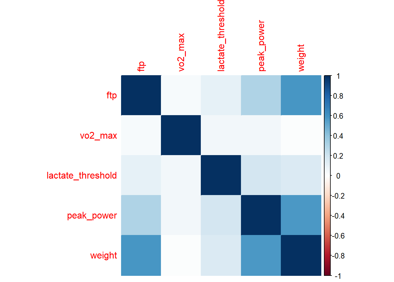
We can see from the above output that Peak Power and functional threshold power are positively correlated with weight. If we just used these values we would always end up with the heavier cyclist coming out on top. If we are looking for a climber this would be detrimental (weight plays a huge role in the mountains), we will therefore normalize our variables for weight.
CyclingDataFilteredDF <- CyclingDataFilteredDF %>%
  mutate(
    PeakPower_Kg = peak_power/weight,
    FTP_Kg = ftp/weight)

NumericVarsDF <- CyclingDataFilteredDF %>%
  select_if(is.numeric)
NumericVarsDF<-NumericVarsDF %>%
  select(3,5:8,16,17)
Note how I add the new columns to the CyclingDataFiltered matrix and not NumericVars matrix. I do this so all data is kept together, it’s good practice and easier for when we want to pull in some of the other variables later on.
Now let’s check our correlation again, using only columns 5, 8, 9, 11, and 18-20 of the CyclingDataFiltered. We will print a plot using method="color"
CorrelationMatrix <-cor(NumericVarsDF,use="complete.obs")
CorrelationMatrix
ftp vo2_max lactate_threshold peak_power
ftp 1.00000000 0.03609121 0.10863184 0.30847039
vo2_max 0.03609121 1.00000000 0.05697213 0.05133952
lactate_threshold 0.10863184 0.05697213 1.00000000 0.18570700
peak_power 0.30847039 0.05133952 0.18570700 1.00000000
weight 0.58733982 0.01689525 0.15313930 0.57936304
PeakPower_Kg -0.05953057 0.05592889 0.11069704 0.78472705
FTP_Kg 0.81676466 0.04279823 0.03497664 -0.02185793
weight PeakPower_Kg FTP_Kg
ftp 0.58733982 -0.05953057 0.81676466
vo2_max 0.01689525 0.05592889 0.04279823
lactate_threshold 0.15313930 0.11069704 0.03497664
peak_power 0.57936304 0.78472705 -0.02185793
weight 1.00000000 -0.04014058 0.02496986
PeakPower_Kg -0.04014058 1.00000000 -0.04458851
FTP_Kg 0.02496986 -0.04458851 1.00000000CorrelationMatrix <-cor(NumericVarsDF,use="complete.obs")
corrplot(CorrelationMatrix, method="color")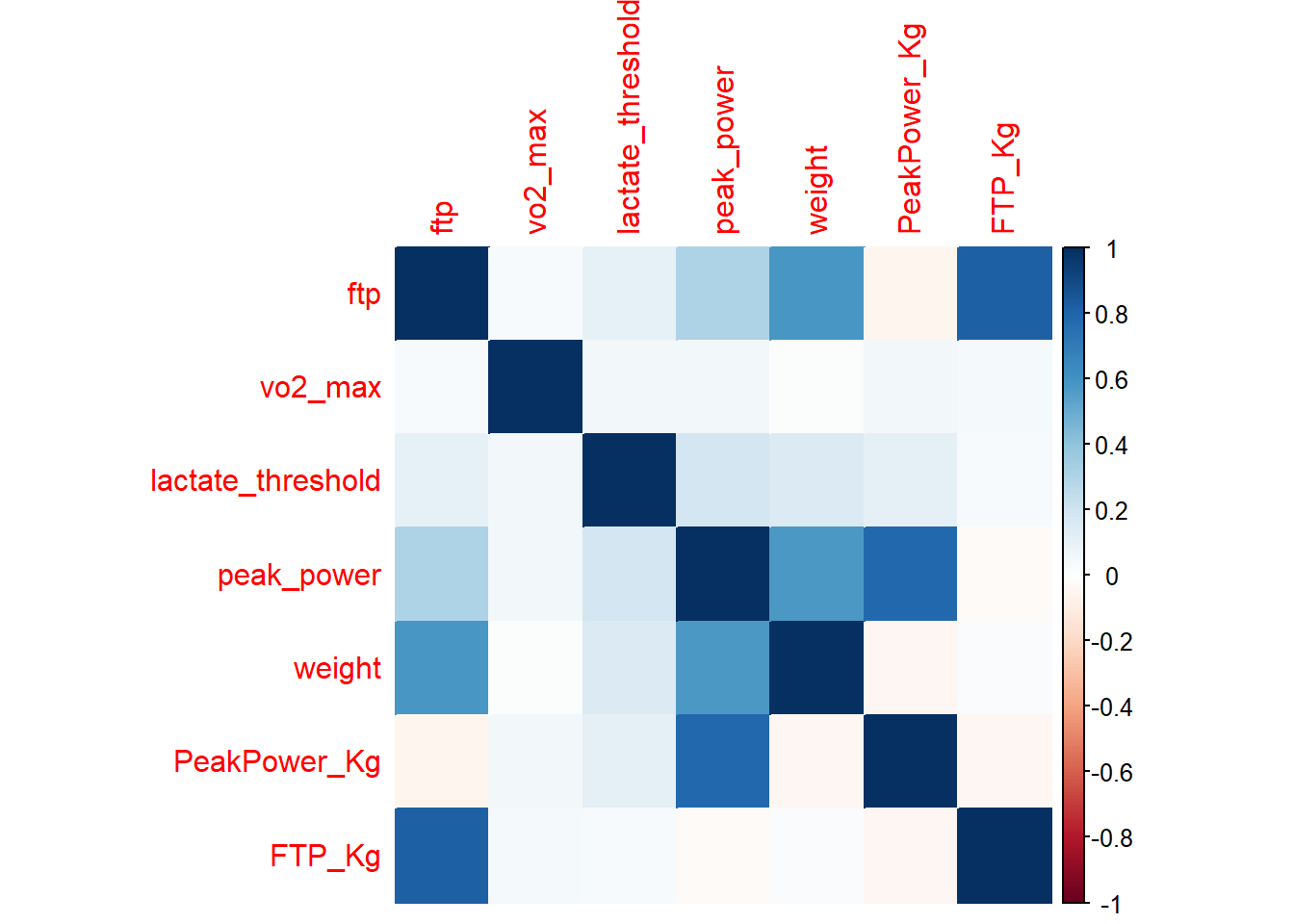
Another way to examine the association between two variables is to plot a scatter plot. Lets plot our original and new power variables against weight and see how they changed.
PPPlot<-ggplot(CyclingDataFilteredDF, aes(peak_power, weight))+
  geom_point() + stat_smooth(method = "lm",
              formula =y ~ x,
              geom = "smooth")
print(PPPlot)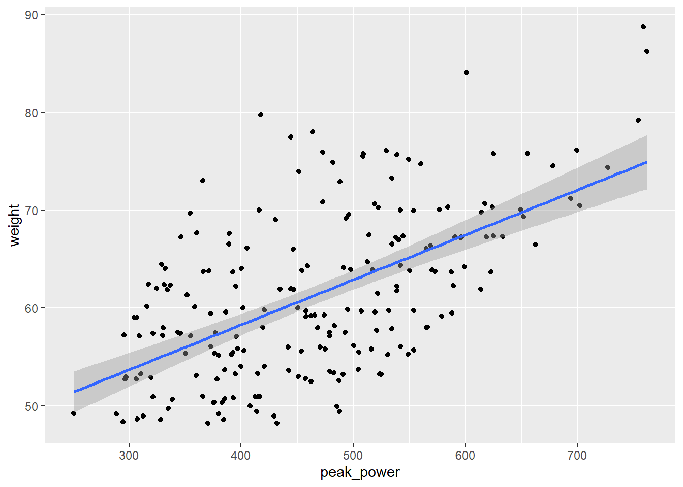
PPKgPlot<-ggplot(CyclingDataFilteredDF, aes(PeakPower_Kg, weight))+
geom_point()+
  geom_point() + stat_smooth(method = "lm",
              formula =y ~ x,
              geom = "smooth")
print(PPKgPlot)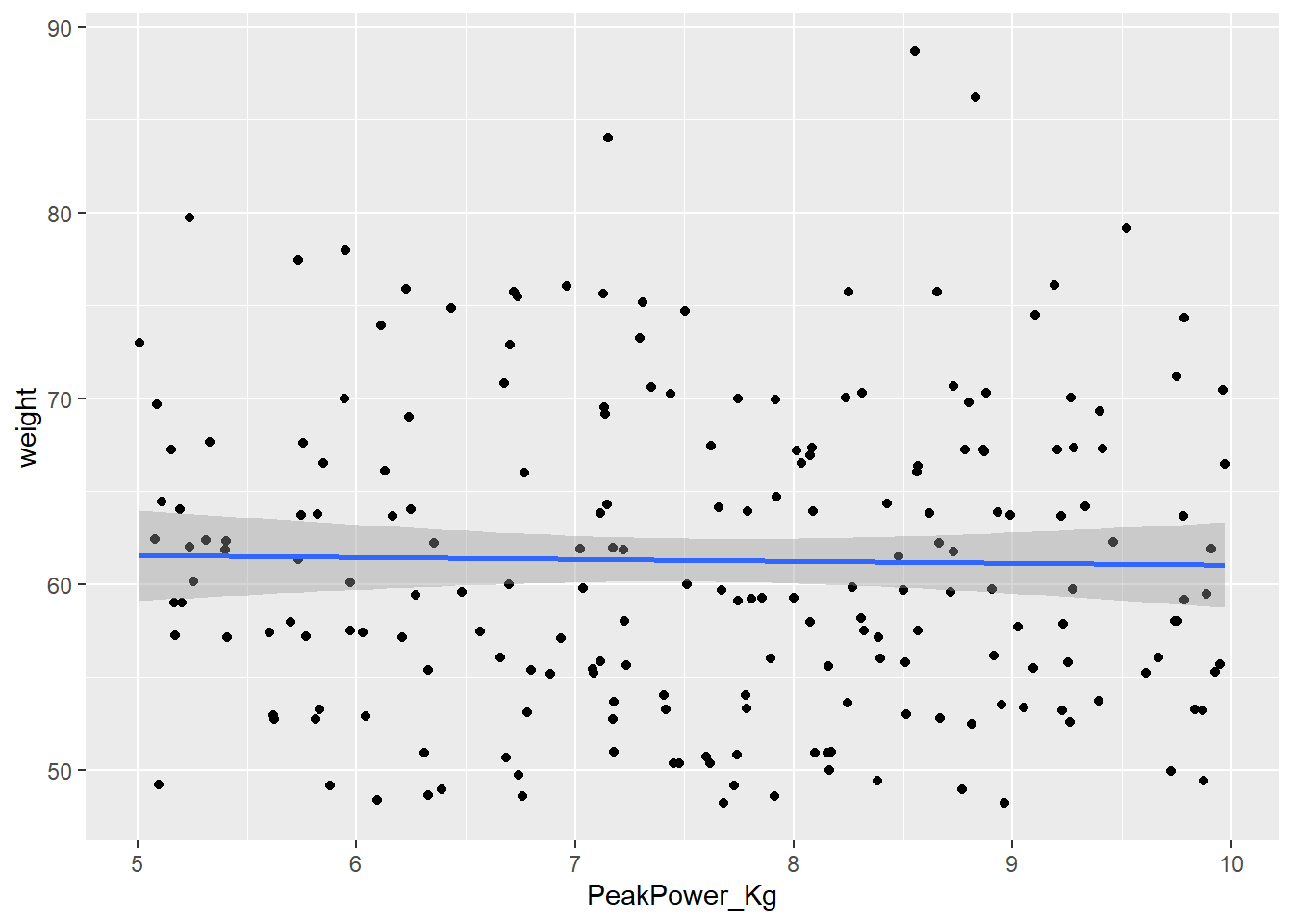
FTPPlot<-ggplot(CyclingDataFilteredDF, aes(ftp, weight))+
geom_point()+
  geom_point() + stat_smooth(method = "lm",
              formula =y ~ x,
              geom = "smooth")
print(FTPPlot)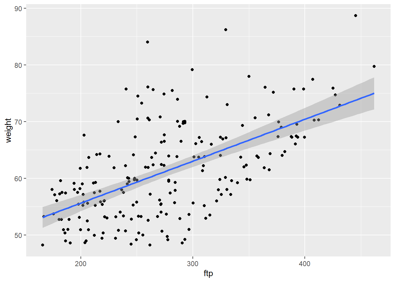
FTPKgPlot<-ggplot(CyclingDataFilteredDF, aes(FTP_Kg, weight))+
geom_point()+
  geom_point() + stat_smooth(method = "lm",
              formula =y ~ x,
              geom = "smooth")
print(FTPKgPlot)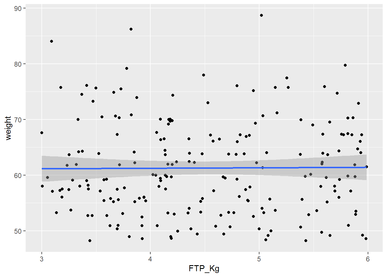
Looking at the correlation matrix we can see that the correlation between weight and our performance outcomes has disappeared. We can now compare these indicators per kg body weight which means we can make a fairer comparison between athletes, especially when looking for climbers.
Using the descr function which is part of the summarytools package is an easy way to create a quick descriptive overview table of your data.
DescriptiveTable <- descr(CyclingDataFilteredDF[,c(4:19)])
print(DescriptiveTable)
Descriptive Statistics
CyclingDataFilteredDF
N: 207
Age anxiety attention ftp FTP_Kg height lactate_threshold
----------------- -------- --------- ----------- -------- -------- -------- -------------------
Mean 15.79 9.74 65.23 276.41 4.51 169.08 301.51
Std.Dev 0.73 5.88 20.81 66.03 0.86 14.24 29.83
Min 15.00 0.00 30.00 165.99 3.00 132.30 218.26
Q1 15.00 5.00 46.00 220.96 3.76 158.40 283.41
Median 16.00 10.00 66.00 270.79 4.40 167.70 304.09
Q3 16.00 15.00 81.00 322.75 5.25 176.60 319.75
Max 17.00 20.00 100.00 461.62 5.99 218.50 379.01
MAD 1.48 7.41 28.17 74.12 1.03 13.34 27.63
IQR 1.00 10.00 35.00 100.80 1.44 18.00 36.24
CV 0.05 0.60 0.32 0.24 0.19 0.08 0.10
Skewness 0.35 0.04 0.00 0.51 0.13 0.49 -0.19
SE.Skewness 0.17 0.17 0.17 0.17 0.17 0.17 0.17
Kurtosis -1.09 -1.11 -1.26 -0.46 -1.20 0.56 -0.03
N.Valid 207.00 207.00 207.00 207.00 207.00 207.00 206.00
Pct.Valid 100.00 100.00 100.00 100.00 100.00 100.00 99.52
Table: Table continues below
peak_power PeakPower_Kg self_efficacy technical_skill vo2_max weight
----------------- ------------ -------------- --------------- ----------------- --------- --------
Mean 465.49 7.60 25.28 5.56 60.48 61.29
Std.Dev 107.21 1.40 9.19 2.91 9.18 8.42
Min 250.81 5.01 10.00 1.00 41.90 48.21
Q1 379.74 6.39 17.00 3.00 53.08 55.20
Median 462.43 7.68 26.00 6.00 61.33 59.73
Q3 539.01 8.77 33.00 8.00 67.57 67.24
Max 761.63 9.97 40.00 10.00 87.24 88.69
MAD 116.03 1.66 11.86 4.45 11.11 9.47
IQR 159.17 2.34 16.00 5.00 14.49 12.02
CV 0.23 0.18 0.36 0.52 0.15 0.14
Skewness 0.41 -0.12 -0.11 0.05 0.14 0.56
SE.Skewness 0.17 0.17 0.17 0.17 0.17 0.17
Kurtosis -0.36 -1.08 -1.19 -1.27 -0.55 -0.17
N.Valid 207.00 207.00 207.00 207.00 201.00 207.00
Pct.Valid 100.00 100.00 100.00 100.00 97.10 100.00
Table: Table continues below
wins_national wins_regional years_experience
----------------- --------------- --------------- ------------------
Mean 8.43 13.55 5.43
Std.Dev 5.32 8.22 2.81
Min 0.00 0.00 1.00
Q1 4.00 7.00 3.00
Median 8.00 13.00 5.00
Q3 12.00 20.00 8.00
Max 20.00 30.00 10.00
MAD 5.93 10.38 2.97
IQR 8.00 13.00 5.00
CV 0.63 0.61 0.52
Skewness 0.43 0.21 0.02
SE.Skewness 0.17 0.17 0.17
Kurtosis -0.70 -1.06 -1.25
N.Valid 207.00 207.00 207.00
Pct.Valid 100.00 100.00 100.00Say we were interested in finding the best climbers for our cycling team and we knew that FTP_kg and vo2_max were two main predictors of cycling success. We could use our descriptive table above and filter for the top quartile of those variables using cut-offs of 5.25 watts/kg and 67.57 ml/min/kg. Similarly if we had historical data we could use descriptives like this to create benchmarks.
TopCyclistDF <- CyclingDataFilteredDF %>%
  filter(FTP_Kg>5.25 & vo2_max>67.57)
We can now see 11 of these athletes meet our criteria. We could choose to rank these players based on their FTP_Kg and VO2_max and print the output.
TopCyclistDF <- TopCyclistDF%>%
  arrange(desc(FTP_Kg), vo2_max) %>%
  mutate(rankingFTP = rank(desc(FTP_Kg)),
         rankingVO2 = rank(desc(vo2_max)))
print(TopCyclistDF)
# A tibble: 11 × 21
Cyclist_ID Date_of_Birth Gender Age ftp anxiety vo2_max lactate_threshold
<int> <date> <chr> <int> <dbl> <int> <dbl> <dbl>
1 290 2007-10-24 Male 15 315. 17 70.6 316.
2 463 2006-10-12 Male 16 351. 4 75.9 314.
3 394 2007-06-29 Male 16 364. 3 72.2 304.
4 467 2006-07-05 Male 17 392. 12 71.6 335.
5 540 2007-03-09 Male 16 278. 18 70.4 292.
6 246 2006-11-08 Male 16 358. 17 76.0 268.
7 415 2008-01-09 Male 15 357. 10 70.8 293.
8 342 2007-04-04 Male 16 346. 14 74.4 312.
9 577 2006-01-22 Male 17 297. 9 71.3 322.
10 532 2008-06-04 Male 15 300. 6 67.7 301.
11 482 2007-02-01 Male 16 407. 17 71.7 324.
# ℹ 13 more variables: peak_power <dbl>, weight <dbl>, height <dbl>,
# years_experience <int>, technical_skill <int>, self_efficacy <int>,
# attention <int>, wins_national <int>, wins_regional <int>,
# PeakPower_Kg <dbl>, FTP_Kg <dbl>, rankingFTP <dbl>, rankingVO2 <dbl>Alternatively we could choose to create a visual radar plot to compare athletes. I will show you how to do this but do not worry if it looks complicated, you will get more practice in creating plots like this during your data visualisation class in semester 2.
We first will need to ensure the data we are interested in is normalized on a scale of 0-1. If we do not do this we would not be able to detect differences in variables with small outcome values. So let’s say we want to display the athletes years_experience, age, VO2_max, FTP_Kg and lactate_threshold.
# Define the columns to normalize
ColumnsToNormalize <- c("Age","vo2_max","lactate_threshold","years_experience","FTP_Kg")


CyclingDataFilteredDF <- CyclingDataFilteredDF %>%
  mutate(across(all_of(ColumnsToNormalize), ~ . / max(., na.rm = TRUE), .names = "Norm_{col}"))

# Add the normalized columns back to the TopCyclist data frame
TopCyclistDF <- CyclingDataFilteredDF %>%
  filter(FTP_Kg>5.25 & vo2_max>67.57)

TopCyclistDF <- TopCyclistDF%>%
  arrange(desc(FTP_Kg), vo2_max) %>%
  mutate(rankingFTP = rank(desc(FTP_Kg)),
         rankingVO2 = rank(desc(vo2_max)))

# Filter for specific rider or riders in this case we will take the best based on VO2max and the number 10 based on VO2max
RidersDF <- TopCyclistDF %>%
filter(rankingVO2==1 | rankingVO2 ==10)

# I take the data columns I want to use
RadarDataDF <- RidersDF[,c("Norm_years_experience", "Norm_Age", "Norm_vo2_max", "Norm_FTP_Kg", "Norm_lactate_threshold", "Cyclist_ID")]

# Add two more rows with the max value = 1 and the min value = 0, this is so we can set the boundaries of the radar.
RadarDataDF <- data.frame(years_experience = c(1, 0, RadarDataDF$Norm_years_experience),
Age = c(1, 0, RadarDataDF$Norm_Age),
Vo2_max = c(1, 0, RadarDataDF$Norm_vo2_max),
FTP_Kg = c(1, 0, RadarDataDF$Norm_FTP_Kg),
Lactate_threshold = c(1,0, RadarDataDF$Norm_lactate_threshold),
row.names=c("max","min",as.character(RadarDataDF$Cyclist_ID)))

# Create the radar chart
RadarPlot <- radarchart(
  RadarDataDF)

legend(-2,0,
       legend=c("P1","P10"),
       pch=c(15,16),
       col=c("red","black"),
       lty=c(1,2))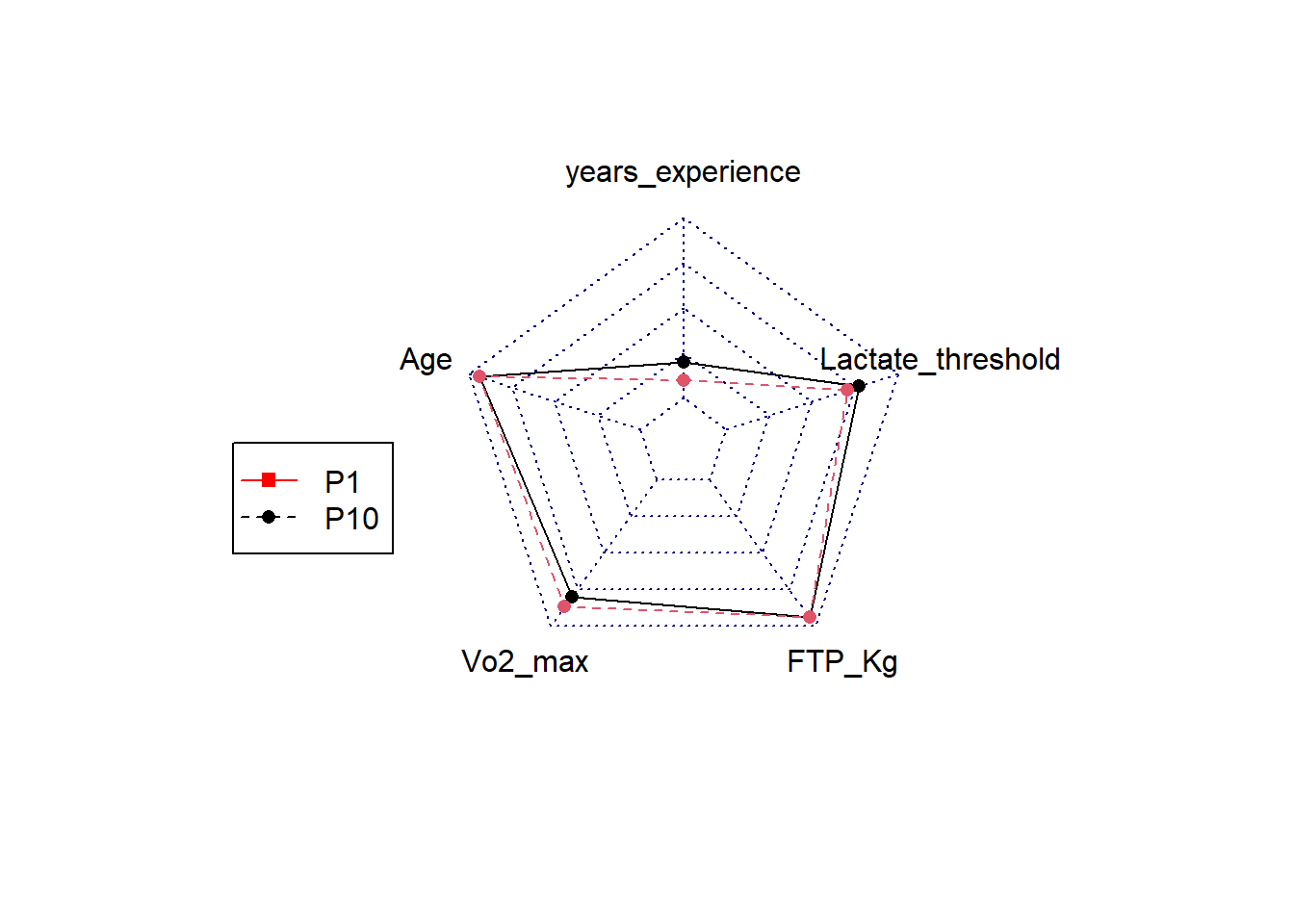
# Print the radar chart
print(RadarPlot)NULLAbove we used the data and ranked cyclist based on some outcomes we know or think are important. However, if we want to advance from this we could run predictive analysis to discover what determines wins as a sprinter, climber or classic rider. To conduct predictive analysis we will ideally need a historical data set to develop our model. This means we need a data set which has: 1) the exposure measures (i.e. those that potentially predict the outcome), 2) the performance outcome measure (i.e. in our case the number of wins), 3) additional categorisation variable (i.e. in our case whether or not the cyclists became a classic rider, sprinter or grant tour rider).
Let’s use the “CyclingTI_predictive.csv” sample data set on myplace to show you how predictive analysis could work. The data can also be read in via the following shared link:
rm(list=setdiff(ls(), "CyclingDataFilteredDF"))

FilePath <- "https://strath-my.sharepoint.com/:x:/g/personal/xanne_janssen_strath_ac_uk/Ee0zURhgzfNOo4NulEhOMmwBCBCrPWAq-UOFbP7WqQolEw?download=1"

CyclingDataPredictiveDF <- as_tibble(read.csv(FilePath))

CyclingDataPredictiveDF <- CyclingDataPredictiveDF %>%
  filter(Gender == "Male")
If you have inspected the data you will have seen that Peak Power and FTP are not normalised for weight. Let’s do this.
CyclingDataPredictiveDF <- CyclingDataPredictiveDF %>%
  mutate(
    PeakPower_Kg = peak_power/weight,
    FTP_Kg = ftp/weight)

CyclingDataPredictiveDF <- CyclingDataPredictiveDF %>%
  arrange(Cyclist_ID)
Now we are ready to ready to create a predictive model. We will create predictions for sprint wins.
In B1700 you will go over an introduction into predictive analysis using linear regression and in semester 2 you will delve into this even more. We will use the same method (lm() function) and use sprint_wins as outcome. FTP_Kg, vo2_max, Lactate_Threshold, PeakPower_Kg, anxiety, height, weight, self_efficacy,attention, technical_skill will be our predictor variables.
# Sprint wins
set.seed(123)
TrainIndex <- createDataPartition(CyclingDataPredictiveDF$sprint_wins, p=0.8, list=FALSE, times=1)
TrainDataDF <- CyclingDataPredictiveDF[TrainIndex, ]
TestDataDF <- CyclingDataPredictiveDF[-TrainIndex, ]

# Model with all variables
WinsPredictionSprintDF <- lm(sprint_wins ~ FTP_Kg + vo2_max + lactate_threshold + PeakPower_Kg + anxiety + height + weight+ self_efficacy + attention + technical_skill, data = TrainDataDF)
summary(WinsPredictionSprintDF)
Call:
lm(formula = sprint_wins ~ FTP_Kg + vo2_max + lactate_threshold +
    PeakPower_Kg + anxiety + height + weight + self_efficacy +
    attention + technical_skill, data = TrainDataDF)

Residuals:
    Min      1Q  Median      3Q     Max
-4.5615 -1.2002 -0.1318  0.9247  5.3863

Coefficients:
                    Estimate Std. Error t value Pr(>|t|)
(Intercept)       -16.034141   1.166630 -13.744  < 2e-16 ***
FTP_Kg              0.481121   0.161956   2.971  0.00312 **
vo2_max             0.003589   0.008210   0.437  0.66224
lactate_threshold   0.004507   0.002074   2.173  0.03026 *
PeakPower_Kg        1.394005   0.108679  12.827  < 2e-16 ***
anxiety             0.034100   0.013579   2.511  0.01237 *
height              0.015252   0.035215   0.433  0.66514
weight              0.092748   0.036756   2.523  0.01195 *
self_efficacy       0.002022   0.008976   0.225  0.82191
attention          -0.006599   0.003906  -1.689  0.09179 .
technical_skill     0.051158   0.027979   1.828  0.06812 .
---
Signif. codes:  0 '***' 0.001 '**' 0.01 '*' 0.05 '.' 0.1 ' ' 1

Residual standard error: 1.777 on 470 degrees of freedom
Multiple R-squared:  0.5931,    Adjusted R-squared:  0.5844
F-statistic: 68.5 on 10 and 470 DF, p-value: < 2.2e-16#Model with just sign variables
WinsPredictionSprintDF_sign <- lm(sprint_wins ~ FTP_Kg + lactate_threshold+ PeakPower_Kg+anxiety+weight, data = TrainDataDF)
summary(WinsPredictionSprintDF_sign)
Call:
lm(formula = sprint_wins ~ FTP_Kg + lactate_threshold + PeakPower_Kg +
    anxiety + weight, data = TrainDataDF)

Residuals:
    Min      1Q  Median      3Q     Max
-4.6474 -1.2743 -0.1421  1.0404  5.5104

Coefficients:
                    Estimate Std. Error t value Pr(>|t|)
(Intercept)       -15.851358   0.914921 -17.325  < 2e-16 ***
FTP_Kg              0.474710   0.162097   2.929  0.00357 **
lactate_threshold   0.004671   0.002071   2.256  0.02453 *
PeakPower_Kg        1.401687   0.108676  12.898  < 2e-16 ***
anxiety             0.032559   0.013522   2.408  0.01643 *
weight              0.108124   0.010308  10.489  < 2e-16 ***
---
Signif. codes:  0 '***' 0.001 '**' 0.01 '*' 0.05 '.' 0.1 ' ' 1

Residual standard error: 1.779 on 475 degrees of freedom
Multiple R-squared:  0.5875,    Adjusted R-squared:  0.5832
F-statistic: 135.3 on 5 and 475 DF, p-value: < 2.2e-16# Model with just one variable
WinsPredictionSprint_PP <- lm(sprint_wins ~ PeakPower_Kg, data = TrainDataDF)
summary(WinsPredictionSprint_PP)
Call:
lm(formula = sprint_wins ~ PeakPower_Kg, data = TrainDataDF)

Residuals:
   Min     1Q Median     3Q    Max
-4.567 -1.509 -0.378  1.219  7.520

Coefficients:
             Estimate Std. Error t value Pr(>|t|)
(Intercept)   -6.3371     0.5599  -11.32   <2e-16 ***
PeakPower_Kg   1.6173     0.1002   16.14   <2e-16 ***
---
Signif. codes:  0 '***' 0.001 '**' 0.01 '*' 0.05 '.' 0.1 ' ' 1

Residual standard error: 2.22 on 479 degrees of freedom
Multiple R-squared:  0.3522,    Adjusted R-squared:  0.3508
F-statistic: 260.4 on 1 and 479 DF, p-value: < 2.2e-16# Predict on testing data
Predictions_sign <- predict(WinsPredictionSprintDF_sign, newdata = TestDataDF)
Predictions_PP <- predict(WinsPredictionSprint_PP, newdata = TestDataDF)
# Evaluate models performance
mse <- mean((TestDataDF$sprint_wins-Predictions_sign)^2)
rmse<-sqrt(mse)
print(rmse)[1] 1.947354mse <- mean((TestDataDF$sprint_wins-Predictions_PP)^2)
rmse<-sqrt(mse)
print(rmse)[1] 2.270797From the output above we see that to win sprint wins there are several significant predictors. We also saw that if we only use one of these significant predictors our model accuracy goes down (decrease in R-square and increase in RMSE). We could use this information to update our previous visualisations and rankings. However, another way in which we can use the dataset and make decisions on riders is to create a decision tree (predictive analysis). A decision tree can tell us if a rider is most likely to succeed in becoming for example a world performing sprinter. A simple version of this can be created as follows.
We will create a new training and test data set but this time we use the raw data, we do not need to normalise our data.
# First lets create a criteria to indicate top sprinters versus those that are not. We will use more than 5 wins as a criteria for being a sprinter.

CyclingDataPredictiveDF <- CyclingDataPredictiveDF %>%
mutate(Sprinter = ifelse(sprint_wins>5,1,0))

# Create training and test data set
set.seed(1)
TrainIndex <- createDataPartition(CyclingDataPredictiveDF$Sprinter, p=0.8, list=FALSE, times=1)
TrainDataDF <- CyclingDataPredictiveDF[TrainIndex, ]
TestDataDF <- CyclingDataPredictiveDF[-TrainIndex, ]
Next we like to check if the probability of becoming a sprinter are the same in both datasets.
prop.table(table(TestDataDF$Sprinter))
        0         1
0.8166667 0.1833333 prop.table(table(TrainDataDF$Sprinter))
        0         1
0.8395833 0.1604167
We can see that the percentages of becoming a sprinter (1) or not (0) are very similar in both sets. This means we are ready to build our model.
library(rpart.plot)
library(rpart)

fit <- rpart(Sprinter~ FTP_Kg + lactate_threshold+ PeakPower_Kg+anxiety+weight+technical_skill, data = TrainDataDF, method = 'class')
rpart.plot(fit)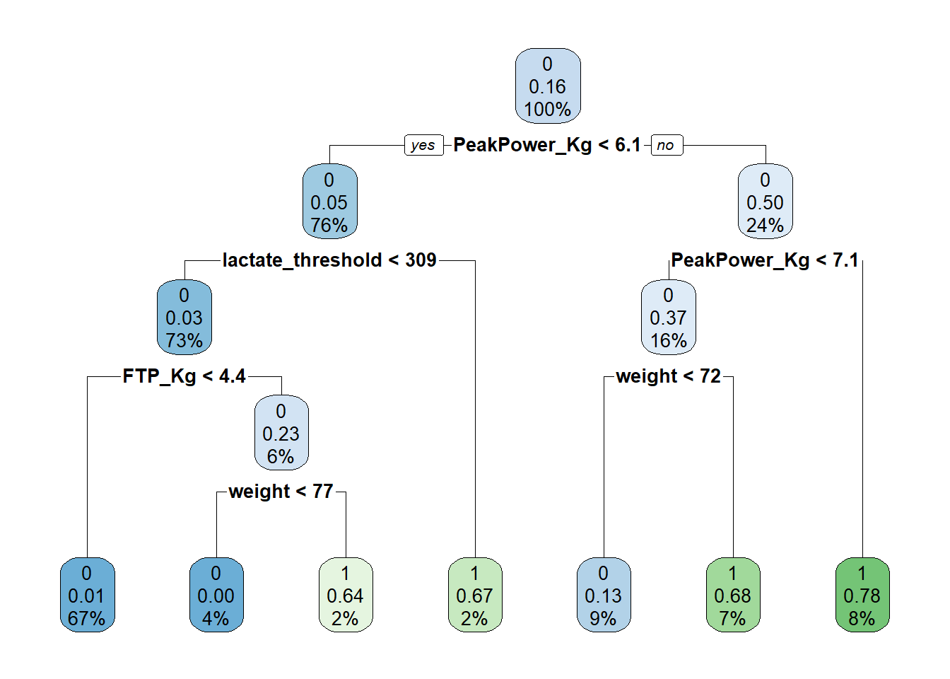
# Left indicates yes, right indicates no.We have now build a decision tree using the KPIs we identified earlier via regression analysis. Peak power comes out as the most important variable which is in line with what we found in our regression analysis. What we see in this tree is at the first node there is 16% predicted chance of becoming a sprinter (this is without taking anything into account). If peak power per KG body weight is greater than 6.1 the predicted likelihood goes up to 50% (24% of our sample is included in this node), if peak power is greater than 7.1 chances go up to 78%. If peak power is less than 7.1 but a riders weight is greater than 72kg, there is a 68% chance of becoming a sprinter, whereas if weight is less than 72kg, the chances of becoming a sprinter go down to 13%. If however the athletes peak power is less than 6.1 but their lactate threshold is greater than 309 their chance of becoming a sprinter is 67%.
Now we have a model which can predict athletes chances of becoming a sprinter we want to test the accuracy on our test sample.
TestDataDF$prediction <- predict(fit, TestDataDF, type = 'class')

# TP+TN/Total sample
accuracy <- (sum(TestDataDF$Sprinter == 1 & TestDataDF$prediction==1)+sum(TestDataDF$Sprinter == 0 & TestDataDF$prediction==0)) / sum(TestDataDF$Sprinter==1 | TestDataDF$Sprinter==0)

# TP/(TP+FN) - Sensitivity is the ability of a test to correctly identify athletes who do become sprinters
sensitivity <- sum(TestDataDF$Sprinter == 1 & TestDataDF$prediction==1) / (sum(TestDataDF$Sprinter==1 & TestDataDF$prediction ==1) ++sum(TestDataDF$Sprinter == 1 & TestDataDF$prediction==0))

# TN/(TN+FP) - Specificity is the ability of a test to correctly exclude athletes who do not become sprinters.
specificity <-  sum(TestDataDF$Sprinter == 0 & TestDataDF$prediction==0) / (sum(TestDataDF$Sprinter==0 & TestDataDF$prediction ==0) ++sum(TestDataDF$Sprinter == 0 & TestDataDF$prediction==1))

cat("accuracy = ", accuracy, "\n")
accuracy = 0.8416667 cat("sensitivity = ", sensitivity, "\n")sensitivity = 0.6818182 cat("specificity = ", specificity, "\n")specificity = 0.877551 Based on the value above, our model appears to be 84.17% accurate, not bad, however it does appear to miss out on identifying potential sprinters (sensitivity 68.18%). Now you could choose to see if you could improve the model slightly or alternatively if you were happy you could apply it to our junior dataset and predict potential up and coming sprinters.
CyclingDataFilteredDF$predictions <- predict(fit, newdata = CyclingDataFilteredDF, type = "class")Exercise 1: If you removed the CyclingDataDF from your environment, reload the CyclingTI.csv file and reassign it to CyclingDataDF. The data can be found here or you can use the following link:
# Set the directory where the CSV files are located
FilePath <- "https://strath-my.sharepoint.com/:x:/g/personal/xanne_janssen_strath_ac_uk/ESWr_kmjIRtIu-5RxgMdzpIBGbBd4jc4nH4wbNXGmmNKeg?download=1"

CyclingDataDF <- as_tibble(read.csv(FilePath))
Exercise 2: Filter your data for boys aged 12 to 14 years. Then check the data (i.e. variable types, inaccurate values) an make any necessary adjustments. Remember a VO2max below 32 is normally only seen in very unfit people or those with a medical condition and we would expect a lactate threshold to be above 100. Deal with any issues
# Filter
CyclingDataFilteredDF <- CyclingDataDF %>%
  filter(Gender == "Male" & Age >= 12 & Age <= 14)

# Change date of birth to date type
CyclingDataFilteredDF <- CyclingDataFilteredDF %>%
      mutate(Date_of_Birth = dmy(Date_of_Birth))

# Check for errors and outliers in each numerical variable
NumericVars <- CyclingDataFilteredDF %>%
  select_if(is.numeric)

for (var in names(NumericVars)) {
  VarSummary <- summary(NumericVars[[var]],na.rm=TRUE)

  # Print summary statistics
  cat("Variable:", var, "\n")
  print(VarSummary)
  cat("\n")
}

# The printout shows some very low VO2 Max values.

# Remove inaccurate values
CyclingDataFilteredDF$vo2_max<-ifelse(CyclingDataFilteredDF$vo2_max<40,NA,CyclingDataFilteredDF$vo2_max)
Exercise 3: Next up let’s focus on the variables we plan to use: ftp, VO2max, lactate threshold, peak power and weight. Create a new dataframe with just these variables and check their normality and correlation and make the appropriate corrections (focus mainly on ftp).
# Select relevant variables.
OutcomesDF<-CyclingDataFilteredDF %>%
  select(5,7:10)

# Create a histogram to visualize the distribution and outliers of our numerical data

for (var in names(OutcomesDF)) {
    histo<-ggplot(data = CyclingDataFilteredDF, aes_string(var)) +
    geom_histogram() +
    ggtitle(paste("Histogram of", var))
  print(histo)
}for (var in names(OutcomesDF)) {
cat(var, "Skewness:", skewness(CyclingDataFilteredDF[[var]],na.rm = TRUE),"\n")
cat(var, "Kurtosis:",kurtosis(CyclingDataFilteredDF[[var]],na.rm=TRUE),"\n")
}
# Examine correlation
CorrelationMatrix <-cor(OutcomesDF,use="complete.obs")
CorrelationMatrix
corrplot(CorrelationMatrix, method= "color")# High correlation between ftp and weight (also between lactate threshold and peak_power but we will ignore this for now)
CyclingDataFilteredDF$ftp_kg <- CyclingDataFilteredDF$ftp/CyclingDataFilteredDF$weight
OutcomesDF$ftp_kg <- OutcomesDF$ftp/OutcomesDF$weightExercise 4: Can you list the top quartile performing riders based on VO2Max. Create a radar plot for the cyclist with the highest VO2max and the one in 20th position (using ftp_kg, vo2_max, lactate_threshold, years_experience, attention).
DescriptiveTable <- descr(CyclingDataFilteredDF[,c(7)])
print(DescriptiveTable)

# Define the columns to normalize
ColumnsToNormalize <- c("ftp_kg","vo2_max","lactate_threshold","years_experience","attention")

CyclingDataFilteredDF <- CyclingDataFilteredDF %>%
  mutate(across(all_of(ColumnsToNormalize), ~ . / max(., na.rm = TRUE), .names = "Norm_{col}"))

# Filter based on top quartile and rank athletes based on VO2 max.
TopCyclistDF <- CyclingDataFilteredDF %>%
  filter(vo2_max>64.94)

TopCyclistDF <- TopCyclistDF%>%
  arrange(desc(vo2_max)) %>%
  mutate(rankingVO2 = rank(desc(vo2_max)))
print(TopCyclistDF)

# Filter for specific rider or riders in this case we will take the best based on VO2max and the number 10 based on VO2max
RidersDF <- TopCyclistDF %>%
filter(rankingVO2==1 | rankingVO2 ==20)

# I take the data columns I want to use
RadarDataDF <- RidersDF[,c("Norm_ftp_kg","Norm_vo2_max","Norm_lactate_threshold","Norm_years_experience","Norm_attention", "Cyclist_ID")]

# Add two more rows with the max value = 1 and the min value = 0, this is so we can set the boundaries of the radar.
RadarDataDF <- data.frame(years_experience = c(1, 0, RadarDataDF$Norm_years_experience),
Attention = c(1, 0, RadarDataDF$Norm_attention),
Vo2_max = c(1, 0, RadarDataDF$Norm_vo2_max),
FTP_Kg = c(1, 0, RadarDataDF$Norm_FTP_Kg),
Lactate_threshold = c(1,0, RadarDataDF$Norm_lactate_threshold),
row.names=c("max","min",as.character(RadarDataDF$Cyclist_ID)))

# Create the radar chart
RadarPlot <- radarchart(
  RadarDataDF)

legend(-2,0,
       legend=c("P20","P1"),
       pch=c(15,16),
       col=c("red","black"),
lty=c(1,2))# Print the radar chart
print(RadarPlot)Exercise 5: Let’s focus on some predictive analysis practice. Load in CyclingTI_predictive.csv and assign it to CyclingDataPredictive. The data can be found here or loaded via:
Once you loaded your data, filter the dataset for males only, and add two columns PeakPower_Kg, FTP_Kg.
FilePath <- "https://strath-my.sharepoint.com/:x:/g/personal/xanne_janssen_strath_ac_uk/Ee0zURhgzfNOo4NulEhOMmwBCBCrPWAq-UOFbP7WqQolEw?download=1"

CyclingDataPredictiveDF <- read.csv(FilePath)

CyclingDataPredictiveDF <- CyclingDataPredictiveDF %>%
  filter(Gender == "Male")

# Calculate variables
CyclingDataPredictiveDF <- CyclingDataPredictiveDF %>%
  mutate(
    PeakPower_Kg = peak_power/weight,
    FTP_Kg = ftp/weight)

CyclingDataPredictiveDF <- CyclingDataPredictiveDF %>%
 arrange(Cyclist_ID)
Exercise 6: Using the predictive data set create a prediction model which predicts grand_tour_wins.
# Note your answer may give slightly different results based on how your data is split but your code should look similar.

# Create training and test data
set.seed(3)
TrainIndex <- createDataPartition(CyclingDataPredictiveDF$grand_tour_wins, p=0.8, list=FALSE, times=1)
TrainDataDF <- CyclingDataPredictiveDF[TrainIndex, ]
TestDataDF <- CyclingDataPredictiveDF[-TrainIndex, ]

# Create a model with all variables using the test data
WinsPredictionTour <- lm(grand_tour_wins ~ FTP_Kg + vo2_max + lactate_threshold + PeakPower_Kg + anxiety + height + weight+ self_efficacy + attention + technical_skill, data = TrainDataDF)
summary(WinsPredictionTour)

# In the above we see only vo2_max is significant, we will run a model with just VO2_max and see what happens to the R-squared.

# Model with just sign variables
WinsPredictionTourVO2 <- lm(grand_tour_wins ~ vo2_max, data = TrainDataDF)
summary(WinsPredictionTourVO2)
# R square remains about the same so a model with just VO2 max should perform as well as a model with all variables included.

# Predict on testing data
PredictionsDF <- predict(WinsPredictionTour, newdata = TestDataDF)
PredictionsVO2DF<-predict(WinsPredictionTourVO2, newdata = TestDataDF)

# Evaluate models performance
mse <- mean((TestDataDF$grand_tour_wins-PredictionsDF)^2)
rmse <- sqrt(mse)
cat("rmse full model = ", rmse, "\n")

mse <- mean((TestDataDF$grand_tour_wins-PredictionsVO2DF)^2)
rmse <- sqrt(mse)
cat("rmse VO2 max = ", rmse, "\n")
Exercise 7: Last let’s create a decision tree displaying the chance of becoming a grand tour winner. Use VO2Max, technical skill, and self_efficacy in your model.
# Create a criteria to indicate grand tour winners versus those that are not. We will use more than 5 wins as a criteria for being a sprinter.

# Check the spread of values to decide on a cut off for potential vs not.
summary(CyclingDataPredictiveDF$grand_tour_wins,na.rm=TRUE)

# Use the third quartile value as splitting threshold
CyclingDataPredictiveDF <- CyclingDataPredictiveDF %>%
mutate(TourRider = ifelse(grand_tour_wins>1,1,0))

# Create training and test data set
set.seed(5)
TrainIndex <- createDataPartition(CyclingDataPredictiveDF$TourRider, p=0.8, list=FALSE, times=1)
TrainDataDF <- CyclingDataPredictiveDF[TrainIndex, ]
TestDataDF <- CyclingDataPredictiveDF[-TrainIndex, ]

# Check distribution in both
prop.table(table(TestDataDF$TourRider))
prop.table(table(TrainDataDF$TourRider))

# Pretty equal so let's move onto creating the model.
GrandTourModel <- rpart(TourRider ~ vo2_max + technical_skill + self_efficacy, data = TrainDataDF, method = 'class')
rpart.plot(GrandTourModel)summary(GrandTourModel)
TestDataDF$prediction <- predict(GrandTourModel, TestDataDF, type = 'class')
# TP+TN/Total sample
accuracy <- (sum(TestDataDF$TourRider == 1 & TestDataDF$prediction==1)+sum(TestDataDF$TourRider == 0 & TestDataDF$prediction==0)) / sum(TestDataDF$TourRider==1 | TestDataDF$TourRider==0)
# TP/(TP+FN) - Sensitivity is the ability of a test to correctly identify athletes who do become sprinters
sensitivity <- sum(TestDataDF$TourRider == 1 & TestDataDF$prediction==1) / (sum(TestDataDF$TourRider==1 & TestDataDF$prediction ==1) ++sum(TestDataDF$TourRider == 1 & TestDataDF$prediction==0))
# TN/(TN+FP) - Specificity is the ability of a test to correctly exclude athletes who do not become sprinters.
specificity <- sum(TestDataDF$TourRider == 0 & TestDataDF$prediction==0) / (sum(TestDataDF$TourRider==0 & TestDataDF$prediction ==0) ++sum(TestDataDF$TourRider == 0 & TestDataDF$prediction==1))
cat("accuracy = ", accuracy, "\n")
cat("sensitivity = ", sensitivity, "\n")
cat("specificity = ", specificity, "\n")```